LLML CS336 Lecture 3.1: Architectures for Transformers

Lecture 3.1: Architecture for Transformer

Introduction

开山鼻祖 Attention is all you need 针对的事机器翻译的问题而提出的，并非完全针对大语言模型。因此，后续大语言模型的调优过程在架构层面做了许多创新性的优化，也带来性能上的大幅度提升。本文将逐一介绍之。

Variations of transformers

Starting with the original transformer…

• (Masked) MultiHead Attention
• Positional Embeddings
• FFN (MLP), with RELU activation function.
• LayerNorm

However, the original transformer is designed for machine translation, which are viewed as a variant of RNNs. Nowadays, different models have different architecture design in detail:

Name	Year	LayerNorm	Parallel Layer	Pre-norm	Position embedding	Activations	Stability tricks
Original transformer	2017	LayerNorm	Serial	❌	Sine	ReLU
GPT	2018	LayerNorm	Serial	❌	Absolute	GeLU
T5 (11B)	2019	RMSNorm	Serial	✅	Relative	ReLU
GPT2	2019	LayerNorm	Serial	❌	Absolute	GeLU
GPT2	2020	RMSNorm	Serial	✅	Relative	GeGLU
T5 (XXL 11B) v1.1	2020	RMSNorm	Serial	✅	Relative	GeGLU
mT5	2020	RMSNorm	Serial	✅	Relative	GeGLU
GPT3 (175B)	2020	LayerNorm	Serial	✅	Absolute	GeLU
GPTJ	2021	LayerNorm	Parallel	✅	RoPE	GeLU
LaMDA	2021				Relative	GeGLU
Anthropic LM (not claude)	2021
Gopher (280B)	2021	RMSNorm	Serial	✅	Relative	ReLU
GPT-NeoX	2022	LayerNorm	Parallel	✅	RoPE	GeLU
BLOOM (175B)	2022	LayerNorm	Parallel	✅	Alibi	GeLU
OPT (175B)	2022	LayerNorm	Serial	❌	Absolute	ReLU
PaLM (540B)	2022	RMSNorm	Parallel	✅	RoPE	SwiGLU	Z-loss
Chinchilla	2022	RMSNorm	Serial	✅	Relative	ReLU
Mistral (7B)	2023	RMSNorm	Serial	✅	RoPE	SwiGLU
LLaMA2 (70B)	2023	RMSNorm	Serial	✅	RoPE	SwiGLU
LLaMA (65B)	2023	RMSNorm	Serial	✅	RoPE	SwiGLU
GPT4	2023			❌
Olmo 2	2024	RMSNorm	Serial	❌	RoPE	SwiGLU	Z-loss, QK-norm
Gemma 2 (27B)	2024	RMSNorm	Serial	✅	RoPE	GeGLU	Logit soft capping, Pre+post norm
Nemotron-4 (340B)	2024	LayerNorm	Serial	✅	RoPE	SqReLu
Qwen 2 (72B) - same for 2.5	2024	RMSNorm	Serial	✅	RoPE	SwiGLU
Falcon 2 11B	2024	LayerNorm	Parallel	✅	RoPE	GeLU	Z-loss
Ph3 (small) - same for ph4	2024	RMSNorm	Serial	✅	RoPE	SwiGLU
Llama 3 (70B)	2024	RMSNorm	Serial	✅	RoPE	SwiGLU
Reka Flash	2024	RMSNorm	Serial	✅	RoPE	SwiGLU
Command R+	2024	LayerNorm	Parallel	✅	RoPE	SwiGLU
OLMo	2024	RMSNorm	Serial	✅	RoPE	SwiGLU
Qwen (14B)	2024	RMSNorm	Serial	✅	RoPE	SwiGLU
DeepSeek (67B)	2024	RMSNorm	Serial	✅	RoPE	SwiGLU
Yi (34B)	2024	RMSNorm	Serial	✅	RoPE	SwiGLU
Mixtral of Experts	2024			❌
Command A	2025	LayerNorm	Parallel	✅	Hybrid (RoPE+NoPE)	SwiGLU
Gemma 3	2025	RMSNorm	Serial	✅	RoPE	GeGLU	Pre+post norm, QK-norm
SmolLM2 (1.7B)	2025	RMSNorm	Serial	✅	RoPE	SwiGLU

Normalization

PreNorm vs PostNorm

Several discussions for PreNorm and PostNorm:

• Discussion

TLDR: With the same parameter settings, pre-norm can be trained more easily than post-norm, however, the final performance does not outweigh post-norm.(or exactly the same for the pre-training process.)

However, for the post-training fine-tuning, the post-normalization architecture has better transfer performance.

However, the gradients of Pre-LN at bottom layers tend to be larger than at top layers, leading to a degradation in performance compared with Post-LN.

But for pre-norm, which can keep the good parts of residual connections, with nicer gradient propagation and fewer spike.

Maybe we can do Double Norm ;)

Layer Norm & RMS Norm

Layer Normalization

在层归一化中，我们沿着 特征维度 ($D$) 计算统计量，对每个 样本 ($N$) 和 序列位置 ($L$) 进行归一化。
这意味着 $\mu$ 和 $\sigma^2$ 是针对每个样本 $n$ 和每个序列位置 $l$ 计算的。

• 均值 $\mu_{n,l}$：

  $$\mu_{n,l} = \frac{1}{D} \sum_{d=1}^D x_{n,l,d}$$

• 方差 $\sigma_{n,l}^2$：

  $$\sigma_{n,l}^2 = \frac{1}{D} \sum_{d=1}^D (x_{n,l,d} - \mu_{n,l})^2$$

• 缩放因子和平移因子： $\gamma$ 和 $\beta$ 在所有样本和序列位置上共享，但通常也是与特征维度 $D$ 相同长度的向量，即 $\gamma, \beta \in \mathbb{R}^{D}$。
  因此，对于每个 $x_{n,l,d}$：

  $$y_{n,l,d} = \gamma_d \left( \frac{x_{n,l,d} - \mu_{n,l}}{\sqrt{\sigma_{n,l}^2 + \epsilon}} \right) + \beta_d$$

在 Transformer 等序列建模模型中，因为序列长度 $N$ 可变（并且是频繁变化），因此为了提升模型的鲁棒性，往往采用 Layer Normalization 的方式实现归一化。

RMS Norm

RMSNorm, which stands for Root Mean Square Normalization, is a layer normalization technique used in some transformer architectures. It’s a simpler and more computationally efficient alternative to traditional Layer Normalization.

The core principle of RMSNorm is to re-scale the activations of a layer based on their root mean square (RMS) value, rather than their mean and standard deviation.

For a given input vector $x$ (the activations from a layer), the RMSNorm operation is defined as:

The normalization also happens in the dimensional feature.

$$y_{n,l,d} = \gamma_d \left( \frac{x_{n,l,d}}{\sqrt{\frac{1}{D} \sum_{i=1}^{D} x_{n,l,i}^2 + \epsilon}} \right)$$

RMSNorm calculates the root mean square, which is essentially the L2 norm divided by the square root of the dimension. This method is simpler as it doesn’t subtract the mean, which is the most computationally expensive part of Layer Normalization. This makes RMSNorm more efficient and faster, especially in large-scale models (Runtime: Memory Movement). It normalizes the magnitude of the activations, which is often sufficient for stabilizing training.

• also: it drops bias terms for memory and optimization stability.

Activations

Activation Functions

For non-linear components in the neural network.

GLU (Gated Activations)

Original Feed Forward Network: $FF(x) = \max(0, xW_1)W_2$.

With GLU:

$$\max(0, xW_1) \to \max(0, xW_1) \otimes (xV)$$

$\otimes$ means element-wise operations, the former part of GLU is also the RELU function, and the latter let the input $x$ passing through the matrix $V$ and controls which message can be passed into this successfully.

$$\text{FF}_{\text{REGLU}}(x) = (\max(0, xW_1) \otimes (xV) ) W_2$$

SwiGLU Mathematical Formula

SwiGLU, which stands for Swish-Gated Linear Unit, is a variant of the Gated Linear Unit (GLU) family. It was introduced by Google Brain in the PaLM model and has since been adopted by other modern large language models, such as LLaMA, as the activation function within their feed-forward networks (FFN). It has been shown to outperform both ReLU and GeLU in terms of performance.

SwiGLU functions as a sub-module within the feed-forward network. Its core idea is to replace the traditional single-path activation with a two-path structure controlled by a “gate.”.

SwiGLU-based FFN:

$$FFN(x) = \text{SwiGLU}(xW_1, xW_2)W_3$$

Here, $x$ is the input vector, and $W_1, W_2, W_3$ are learnable weight matrices.

The core operation of SwiGLU is defined as:

$$\text{SwiGLU}(x, W_1, W_2) = (\text{Swish}(xW_1)) \otimes (xW_2)$$

Where:

• $x$ is the input vector.
• $W_1$ and $W_2$ are two distinct weight matrices.
• $\text{Swish}(\cdot)$ is the activation function defined by:

  $$\text{Swish}(z) = z \cdot \sigma(z)$$

  where $\sigma(z)$ is the Sigmoid function:

  $$\sigma(z) = \frac{1}{1 + e^{-z}}$$

• $\otimes$ denotes element-wise multiplication.

1. Path 1 (Activation Path): The input vector $x$ is multiplied by the weight matrix $W_1$ to produce a vector $z_1 = xW_1$. This vector is then passed through the Swish activation function: Swish($z_1$).
2. Path 2 (Gating Path): The input vector $x$ is multiplied by a separate weight matrix $W_2$ to produce another vector $z_2 = xW_2$.
3. Gating: The result from Path 1, Swish($z_1$), is multiplied element-wise by the result from Path 2,$z_2$.

This element-wise multiplication is the key “gating” mechanism. The second path, $z_2 = xW_2$, acts as a gate, dynamically adjusting the weight of each element in the activated vector from Path 1 based on the input $x$.

• Dynamic Information Flow: The gating design allows the network to learn which features should be amplified or suppressed, providing a more precise way to control information flow. This adaptive gating ability helps the model better capture complex dependencies.
• Smoother Gradients: Unlike ReLU’s hard cutoff (with a gradient of 0 or 1), the Swish function has a smooth gradient. This helps in mitigating the vanishing gradient problem in deep networks, leading to more stable optimization.

Serial vs Parallel layers

Original serialized attention mechanism cannot do parallel computations.

• $y = x + \text{MLP}(\text{LayerNorm}(x + \text{Attention}(\text{LayerNorm}(x))))$
• $y = x + \text{MLP}(\text{LayerNorm}(x)) + \text{Attention}(\text{LayerNorm}(x))$

Positional Embeddings

Basic Positional Encoding

注意力机制抛弃了串行式的词元处理状态，采用并行化的设计而牺牲了序列信息，例如，在计算注意力分数的时候交换不同键值对的位置在形式上对最后的 Attention Score 没有影响，这会影响最后建模的序列性。

因此，需要加入额外的项来表示序列的顺序信息，即在输入中添加 Positional Encoding 来注入绝对的或者相对的位置信息。下面介绍一种最常见的位置编码：基于正余弦的固定位置编码。

输入 $\mathbf{X} \in \mathbb{R}^{n \times d}$，考虑嵌入矩阵 $\mathbf{P} \in \mathbb{R}^{n \times d}$，最终输出的结果是 $\mathbf{X} + \mathbf{P}$。其中：

$$p_{(i, 2j)} = \sin(\frac{i}{10000^{2j/d}}), \ p_{(i, 2j+1)} = \cos(\frac{i}{10000^{2j/d}})$$

绝对位置信息

在二进制中，较高位的交替频率低于较低位，因此，位置编码效仿这样的设计，随着编码维度的增加（列，代表编码位置的不同维度），因此，对于不同的行，（行即代表着序列的原始位置信息），横坐标 $i$ 对应的位置编码矩阵在不同的列 $j$ 下的值都不相同。

$j$ 可以看做控制三角函数的频率信息（以 $i$ 为自变量），而频率不同可以很好的在一个周期性函数上表示非周期的特征，简单来说，每一个行学习到的 p[i, :] 都是不同的。

相对位置信息

使用固定位置编码也可以学习到相对位置的特征，例如一些词组的特定搭配等等，从数学语言解释：对于任何确定的位置偏移量 $\delta$，位置 $\delta + i$ 处的位置编码可以用线性投影 $i$ 处的位置编码通过一个与位置无关的线性投影 $M$ 得到。其中：

$$M = \begin{bmatrix} \cos(\delta\omega_j)& \sin(\delta\omega_j) \\ -\sin(\delta\omega_j) & \cos(\delta\omega_j) \end{bmatrix}$$

上文的线性投影矩阵也具有几何意义，考虑线性变换：

$$\left[\begin{array}{l}x^{\prime} \\y^{\prime}\end{array}\right]=\left[\begin{array}{cc}\cos \left(\delta \omega_{j}\right) & \sin \left(\delta \omega_{j}\right) \\-\sin \left(\delta \omega_{j}\right) & \cos \left(\delta \omega_{j}\right)\end{array}\right]\left[\begin{array}{l}x \\y\end{array}\right]$$

$$\begin{array}{l}x^{\prime}=x \cos \left(\delta \omega_{j}\right)+y \sin \left(\delta \omega_{j}\right) \\y^{\prime}=-x \sin \left(\delta \omega_{j}\right)+y \cos \left(\delta \omega_{j}\right)\end{array}$$

其中 $\omega_j = \frac{1}{10000^{2j/d}}$。

这代表着坐标点 $(x^{\prime}, y^{\prime})$ 是原坐标点 $(x,y)$ 经过旋转 $\delta\omega_j = \frac{\delta}{10000^{2j/d}}$ 个弧度制得来的。在这个语境下，指的是从 $(p_{(i,2j)}, p_{(i, 2j+1)})$ 到 $(p_{(i + \delta,2j)}, p_{(i + \delta, 2j+1)})$ 的线性变换过程。

Dive Deeper into Sine Embeddings

Sine Embeddings, 或者叫做 Sinusoidal Embeddings，是一种对输入向量进行位置编码的方式，这种基于正弦函数的位置编码也是最先在 Attention is all you need 论文中提出的方法。

下文的一些摘录节选自 Transformer 升级之路，并且加上自己的注解。

位置编码重要性不必多言，在自回归模型 Attention Score 计算的过程中，其模型是全对称的，满足恒等式 $f(x,y) = f(y,x)$，这会对最终的序列预测任务造成困扰，因此，需要引入位置编码在学习相关性的基础上学习不同词元的序列特征。而这里的序列特征指的是绝对序列特征和相对序列特征。

为了打破对称性，位置编码改变了自注意力层的函数输入：

$$f'(x) = (\cdots, x_m, \cdots, x_n, \cdots) = f(\cdots, x_m + p_m, \cdots, x_n+p_n, \cdots)$$

这里采用加作为注入位置信息的方式，计算简单并且容易学习，但是也会在训练过程中带来问题，后面会详细讲到这个点。

只考虑这两个位置，并进行泰勒展开：

$$\tilde{f} \approx f + \boldsymbol{p}_m^\top \frac{\partial f}{\partial \boldsymbol{x}_m} + \boldsymbol{p}_n^\top \frac{\partial f}{\partial \boldsymbol{x}_n} + \frac{1}{2} \boldsymbol{p}_m^\top \frac{\partial^2 f}{\partial \boldsymbol{x}_m^2} \boldsymbol{p}_m + \frac{1}{2} \boldsymbol{p}_n^\top \frac{\partial^2 f}{\partial \boldsymbol{x}_n^2} \boldsymbol{p}_n + \underbrace{\boldsymbol{p}_m^\top \frac{\partial^2 f}{\partial \boldsymbol{x}_m \partial \boldsymbol{x}_n} \boldsymbol{p}_n}_{\boldsymbol{p}_m^\top \mathcal{H} \boldsymbol{p}_n}$$

之前的项要么只有 $p_m$，要么只有 $p_n$，要么两个都没有（注意，只有$p$存储了位置信息，$x_n$, $x_m$本身只存储了语义信息），因此表达的是绝对信息。（因为只依赖于单一位置），而最后一项同时出现了 $p_m$ 和 $p_n$，因此这是模型存储相对位置信息的关键。

$\frac{\partial^2 f}{\partial \boldsymbol{x}_m \partial \boldsymbol{x}_n}$ 这一项记为矩阵 $\mathcal{H}$，因此我们的目标项是 $p_m^\top \mathcal{H} p_n = g(m-n)$，而我们需要找到符合条件的编码 $p_m$, $p_n$。

当 $\mathcal{H}$ 为对角矩阵的时候，下面的解可以严格的被表示为 $g(m-n)$，但是对于一般的矩阵，这样的性质是不成立的，我们只能希望 $\mathcal{H}$ 的对角线占主元。

具体的计算过程详见：Original Blog，简直是极为精彩的推导过程！最终，我们从 $d = 2$ 的简单复数情形出发，一步步推导到高维偶数编码的一个可行解：

$$p_m = \begin{pmatrix} \cos m\theta_0 \\ \sin m \theta_0 \\ \cos m \theta_1 \\ \sin n \theta_1 \\ \cdots \\ \cos m \theta_{d/2-1} \\ \sin m \theta_{d/2-1} \end{pmatrix}$$

更深一步，这样的位置编码可以抽象为一种$\beta$进制的编码过程。

一个数 $n$ 在 $\beta$ 进制下的第 $m$ 位：$x_m = \left\lfloor\frac{n}{\beta^{m-1}}\right\rfloor \bmod \beta$

$$\left[\cos \left(\frac{n}{\beta^{0}}\right), \sin \left(\frac{n}{\beta^{0}}\right), \cos \left(\frac{n}{\beta^{1}}\right), \sin \left(\frac{n}{\beta^{1}}\right), \cdots, \cos \left(\frac{n}{\beta^{d / 2-1}}\right), \sin \left(\frac{n}{\beta^{d / 2-1}}\right)\right]$$

$$\beta = 10000^{\frac{2}{d}}$$

取模本质上也是一个周期函数（和 $\sin$,$\cos$如出一辙。）因此，在不同位置的向量做编码，会携带的信息是位置 $n$ 在特定数位进制（$\beta = 10000^{\frac{2}{d}}$ 是一个超参数）下的表示。这样的进制编码信息本身就携带了相对位置信息和绝对位置信息。

• sine embeddings
• absolute embeddings
• relative embeddings
• rope embeddings

Relative positions encoding: $\langle f(x, i), f(y, j) \rangle = g(x, y, i - j)$

Where $\langle .,. \rangle$ means the dot product(which is the attention score) for two different tokens. $g$ is a function which consider relative positional embedding as its input.

For the original sime embeddings: $\text{Embed}(x, i) = v_x + \text{Positional Embedding}(\text{pos})$

$$\begin{aligned} \langle \text{Embed}(x, i), \text{Embed}(y, j) \rangle &= \langle v_x + PE_i, v_y + PE_j \rangle \\ &= \langle v_x, v_y \rangle + \langle v_x, PE_j \rangle + \langle PE_i, v_y \rangle + \langle PE_i, PE_j \rangle \end{aligned}$$

$\langle v_x, v_y \rangle + \langle v_x, PE_j \rangle + \dots$, these are cross-terms that are not relative.

Thus, for the original traditional embeddings, in face of mountains of training data, the model tends to memorize the absolute position instead of the relative position, which would cause a rise of perplexity outside the boundary of training data.

RoPE

Intuition

Unlike the simple adding operation ($v_x + \text{PE}(i)$), RoPE tries to “rotate” the vector, which could perfectly satisfy the “relative position” property.

Consider the most simple situation:

$x = (x_0, x_1) \in \mathbb{R}^2$, we can compute $x'$ with a rotation matrix:

$$R_{\theta}=\left(\begin{array}{cc} \cos \theta & -\sin \theta \\ \sin \theta & \cos \theta \end{array}\right)$$

$$x' = R_\theta x$$

The rotation of angles and doc product will only focus on the relative rotation!

$$\langle R_\alpha a, R_\beta b \rangle = \langle R_{(\alpha - \beta)} a, b \rangle$$

Algorithm

Consider a word vector (we define it as $\{q,k\} = W_{\{q, k\}} x_m$), then we can apply the rotation matrix to the word vector in position $m$:

$$\{q, k\}_m = R_{\Theta, m}^d \cdot \{q, k\}$$

• Before the rotation, the vector does not contain any positional information. (only with semantic meaning)
• After the rotation, the vector contain the positional information with the rotated angle. $\theta_m$
• The core component is the rotation matrix: $R_{\Theta, m}^d$

Of course, we know:

$$R_{\Theta, m}^2= \begin{pmatrix} \cos(m\theta_j) & -\sin(m\theta_j) \\ \sin(m\theta_j) & \cos(m\theta_j) \end{pmatrix}$$

下面的内容用中文，因为太精彩了。

为了简化，我们在后续使用复数运算来代替对二维向量的运算（这两个是等价的），并且我们考虑 $d$ 是一个偶数，这样一个维度为 $d$ 的高维向量就可以被切割为 $\frac{d}{2}$ 个二维向量。（对于 $q$ 和 $k$）

令 $N = \frac{d}{2}$，则原始的高维向量就被表示为了 $N$ 个复数表示：$\{z_1, z_2, \dots, z_j, \dots, z_N\}$, $z_j = x_{2j-1} + x_{2j} i$

则旋转的过程可以表示为：

$$z_j' = z_j \cdot e^{im\theta_j}$$

$$\theta_j = \frac{1}{10000^{2(j-1)/d}}$$

来一点数学：

$$z_{j}^{\prime}=z_{j} \cdot e^{i m \theta_{j}}=\left(x_{2 j-1}+i x_{2 j}\right)\left(\cos \left(m \theta_{j}\right)+i \sin \left(m \theta_{j}\right)\right)$$

$$z_{j}^{\prime}=\left(x_{2 j-1} \cos \left(m \theta_{j}\right)-x_{2 j} \sin \left(m \theta_{j}\right)\right)+i\left(x_{2 j-1} \sin \left(m \theta_{j}\right)+x_{2 j} \cos \left(m \theta_{j}\right)\right)$$

其实，这就是一个二维向量 $(x_{2j-1}, x_{2j})$ 在施加旋转矩阵 $R_{\Theta, m}^2$之后的结果。

最终把向量的维度整合，$\{q,k\}_m$ 的结果就是对 $N$ 个二维向量分别施加旋转矩阵之后的结果，这些二维矩阵因为 $j = 1,2,\dots, N$ 的选择取值不同因此带来旋转的角度也不同。

当然，实际过程中不会具体地做高维向量的切割和合并，而是整合成一个大的分块矩阵：

$$\mathbf{R}_{\Theta,m}^d = \begin{pmatrix} \cos(m\theta_1) & -\sin(m\theta_1) & 0 & 0 & \dots \\ \sin(m\theta_1) & \cos(m\theta_1) & 0 & 0 & \dots \\ 0 & 0 & \cos(m\theta_2) & -\sin(m\theta_2) & \dots \\ 0 & 0 & \sin(m\theta_2) & \cos(m\theta_2) & \dots \\ \vdots & \vdots & \vdots & \vdots & \ddots \end{pmatrix} \in \mathbb{R}^{d \times d}$$

在施加旋转位置编码之后的高维向量就携带着相对位置信息进入 Attention 模块进行参数学习。

Proof

RoPE 的精妙之处在于，经过旋转操作后的两个向量 $\mathbf{q}$ 和 $\mathbf{k}$，它们的内积只依赖于它们之间的相对位置 $m-n$。

在注意力机制中，查询向量 $\mathbf{q}$ 和键向量 $\mathbf{k}$ 分别对应位置 $m$ 和 $n$。RoPE 对它们进行旋转操作：

• 旋转后的查询向量：$\mathbf{q}_m = \mathbf{R}_m \mathbf{q}$
• 旋转后的键向量：$\mathbf{k}_n = \mathbf{R}_n \mathbf{k}$

它们之间的内积为：

$$\langle \mathbf{q}_m, \mathbf{k}_n \rangle = \langle \mathbf{R}_m \mathbf{q}, \mathbf{R}_n \mathbf{k} \rangle$$

利用旋转矩阵的性质，即 $\mathbf{R}_m^T = \mathbf{R}_{-m}$，以及 $\mathbf{R}_m^T \mathbf{R}_n = \mathbf{R}_{n-m}$，我们可以得到：

$$\langle \mathbf{R}_m \mathbf{q}, \mathbf{R}_n \mathbf{k} \rangle = \langle \mathbf{q}, \mathbf{R}_m^T \mathbf{R}_n \mathbf{k} \rangle = \langle \mathbf{q}, \mathbf{R}_{n-m} \mathbf{k} \rangle$$

这个结果表明，旋转后向量的内积（即注意力分数）只取决于相对位置 $n-m$，而不是绝对位置 $m$ 和 $n$。这正是 RoPE 能够有效编码相对位置信息的关键。

More Than That…

相关资料参考：

• Paper: Roformer
• Transformer 升级之路之 RoPE 编码
• Transformer 升级之路之 位置编码

Attention Heads Optimization

Perplexity 大语言模型的困惑度

大模型的困惑度（Perplexity）是一种衡量语言模型好坏的重要指标，它量化了模型对一个给定的文本序列预测的不确定性或困惑程度。困惑度越低，说明模型的预测越准确，泛化能力越强。

困惑度是交叉熵（Cross-Entropy）的指数形式，交叉熵（Cross-Entropy）：用于衡量两个概率分布之间的差异。在语言模型中，它衡量的是模型预测的词汇分布与真实词汇分布（通常是独热编码）之间的差异。交叉熵越小，说明模型预测的概率分布与真实分布越接近，模型性能越好。

给定一个包含 $N$ 个词的测试集文本序列 $W = (w_1, w_2, \dots, w_N)$，该序列在语言模型上的困惑度 $PP(W)$ 的定义为：

$$PP(W) = P(w_1, w_2, \dots, w_N)^{-\frac{1}{N}}$$

其中，$P(w_1, w_2, \dots, w_N)$ 是模型对整个序列的联合概率。

这个联合概率可以根据链式法则分解为一系列条件概率的乘积：

$$P(W) = P(w_1) \cdot P(w_2|w_1) \cdot P(w_3|w_1, w_2) \cdots P(w_N|w_1, \dots, w_{N-1})$$

将这个分解后的公式代入，我们得到：

$$PP(W) = \left( \prod_{i=1}^{N} P(w_i|w_1, \dots, w_{i-1}) \right)^{-\frac{1}{N}}$$

直观理解就是模型输出目标句子的概率乘积。乘上 $1/N$ 的指数是为了抵消句子长度对困惑度计算的影响。（对于 $N$ 较大的测试集，肯定最终的概率计算值会更小，但是开根 $1/N$ 后值会变大，使这个指标和序列无关），最后取倒数是为了让困惑度和对应指标成正比（越困惑，模型的数越大）

困惑度通常通过对数形式来计算，这在数值上更稳定。我们先计算平均交叉熵损失 $L(W)$：

$$L(W) = -\frac{1}{N} \sum_{i=1}^{N} \log_2 P(w_i|w_1, \dots, w_{i-1})$$

然后，困惑度就是这个平均交叉熵的 2 的指数：

$$PP(W) = 2^{L(W)}$$

因此，困惑度 = $2^{\text{平均交叉熵}}$。

• 直观理解：困惑度可以被看作是语言模型在每个位置平均面临的**“有效”选择数量**。

  • 为什么？因为困惑度和 $N$ 无关，取 $N=1$，则可以得到联合概率的值为 $1/100$，平均来说就是有100种可能性。
  • 如果一个模型的困惑度是 100，这意味着该模型在预测下一个词时，平均来说有 100 个同样可能的词汇可供选择。
  • 困惑度越低，模型在每个位置的不确定性越小，其预测能力就越强。
  • 困惑度为 1 是最理想的情况，这代表模型每次都以 100% 的概率预测出正确的词，这在现实中是不可能达到的。

• 与模型性能的关系：

  • 低困惑度：意味着模型对测试集数据的分布有很好的理解，能够给出高概率的正确预测，因此它是一个好的模型。
  • 高困惑度：意味着模型对测试集数据的预测能力较差，对下一个词的预测存在很高的不确定性，因此它是一个差的模型。

在实际应用中，由于大模型通常以 token（而不是词）为单位进行处理，所以困惑度计算也通常基于 token 序列。

GQA & MQA

Let consider the compute cost (at inference time) while the input passing the attention layer.

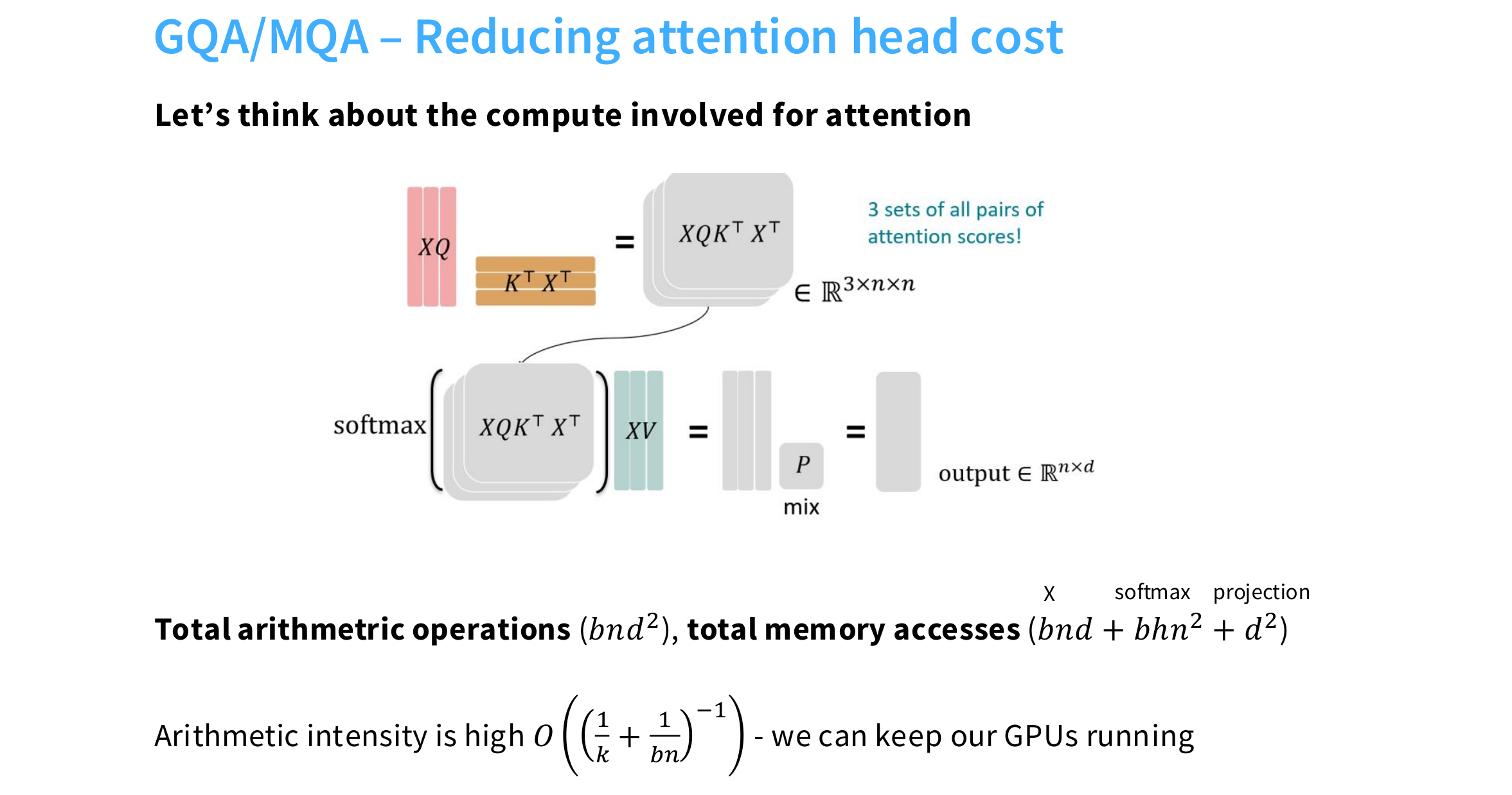
For the input $X$, we first do multi-head attention for transform into $Q,K,V$ matrix in different subspaces.

$$X \in \mathbb{R}^{b \times n \times d}, Q \in \mathbb{R}^{d \times d}$$

For this matrix multiplication, it time complexity is $O(b \times n \times d^2)$

For the total memory access:

• Q, K, V: $\in \mathbb{R}^{d \times d}$

• X and other matrix ($XQ$, $K^\top X^\top$): $\in \mathbb{R}^{b \times n \times d}$

• $XQK^\top X^\top$: $\in \mathbb{R}^{b \times n \times n}$ (And there are $n$ batches)

For the total memory access: $O(bnd + bhn^2 + d^2)$

Arithmetic intensity: $O((\frac{1}{bn} + \frac{1}{d} + \frac{hn}{d^2})^{-1})$

Hence, for text generation task, the generation is done step by step, we need to update the QKV matrices every time, it is quite memory-consuming! But for the generated text, some part of the matrix remain unchanged, thus we can use the cache to store it! KVcache

KV cache

The KV Cache optimizes autoregressive inference by exploiting the structure of the self-attention mechanism.

The core of the attention mechanism is:

$$Attention(Q, K, V) = \text{Softmax}\left(\frac{QK^T}{\sqrt{d_k}}\right)V$$

Where $Q$, $K$, and $V$ are matrices derived from the input sequence $X$.

In autoregressive generation, the model predicts one token at a time. To predict the $i$-th token, the input is the entire sequence from token 1 to $i$. The model would need to compute new $K$ and $V$ matrices for the entire sequence at each step, even though the $K$ and $V$ vectors for the first $i-1$ tokens have already been calculated. This leads to redundant computations.

The KV Cache Solution:
The mathematical principle is based on a simple observation: at each step, a new token is added, which contributes only one new row to the $Q$, $K$, and $V$ matrices. The $K$ and $V$ vectors from previous tokens remain constant.

KV Cache leverages this by:

1. Caching Past Vectors: After computing the $K$ and $V$ vectors for tokens $1$ to $i-1$, these vectors are stored in memory (the “cache”).
2. Efficient Update: To generate the $i$-th token, the model only needs to compute the new $K_i$ and $V_i$ vectors for the current token.
3. Concatenation: The new vectors are concatenated with the cached past vectors to form the full $K$ and $V$ matrices for the current step:

   K_{full} = [K_{cache}, K_i]$$ $$V_{full} = [V_{cache}, V_i]

4. Optimized Computation: The attention score is then calculated using only the new query vector $Q_i$ and the full, concatenated $K$ and $V$ matrices:

   $$Attention_{new} = \text{Softmax}\left(\frac{Q_i K_{full}^T}{\sqrt{d_k}}\right)V_{full}$$

In essence, KV Cache uses memory (space) to store previously computed $K$ and $V$ vectors, eliminating the need to re-compute them in each generation step. This significantly reduces the computational complexity from being a quadratic function of sequence length to a linear one, drastically speeding up inference.

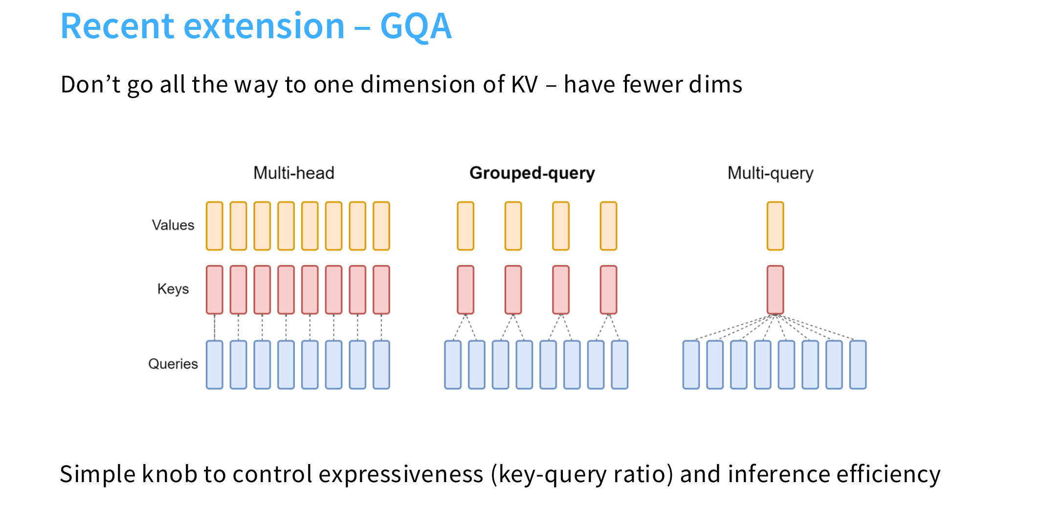
MQA: Multi-Query Attention

对于多头注意力机制，在推理阶段使用内存的空间复杂度为：$O(hnd)$

为了减少内存占用率，MQA实现了从 Multi-Head 到 Multi-Query 的转化，即对于多个头不再使用不同的KV矩阵，而是使用相同的，只是对应的query有不同，这样可以把推理的空间复杂度降一个维度：$O(nd)$。

这样的设定机制是为了搭配 KVcache 的缓存技巧

但是这样会存在问题！在一开始的多头注意力中，原始的输入被线性映射到不同的子空间，按理来说其对应的KV矩阵也应该不同，而不能相同，因此这会带来预测上性能的下降。(相当于丢弃参数了)

因此：GQA 作为一种折中的方案出现了！

GQA

Just a trade of between the expressiveness of the model and the inference efficiency of the model.

Sparse Attention

Attending to the entire context can be expensive (quadratic). Build sparse / structured attention that trades off expressiveness vs runtime (GPT3)

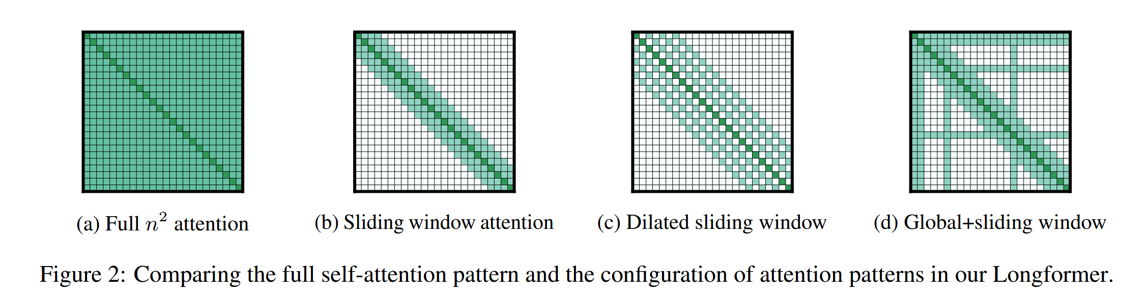
对于传统的 Attention 模块，存在一个非常严重的时间瓶颈：当序列长度 $N$ 变得非常大的时候，注意力矩阵的时间复杂度计算达到了 $O(N^2)$ 级别。因此，同样为了达到 tradeoff（推理性能和推理时间的权衡），稀疏注意力在计算注意力分数时，只让每个 Token 关注序列中的一小部分其他 Token，而不是所有 Token。

稀疏注意力通过定义一个注意力掩码（attention mask）来实现，这个掩码会阻止一些不必要的注意力计算，只保留那些被认为最重要的连接。

Sliding Window Attention

有点类似于 CNN，构建滑动窗口，只捕捉序列滑动窗口的信息。但是这也让其难以捕捉长距离依赖关系。

LongFormer

https://arxiv.org/abs/2004.05150

Transformer-based models are unable to process long sequences due to their self-attention operation, which scales quadratically with the sequence length. To address this limitation, we introduce the Longformer with an attention mechanism that scales linearly with sequence length, making it easy to process documents of thousands of tokens or longer. Longformer’s attention mechanism is a drop-in replacement for the standard self-attention and combines a local windowed attention with a task motivated global attention. Following prior work on long-sequence transformers, we evaluate Longformer on character-level language modeling and achieve state-of-the-art results on text8 and enwik8. In contrast to most prior work, we also pretrain Longformer and finetune it on a variety of downstream tasks. Our pretrained Longformer consistently outperforms RoBERTa on long document tasks and sets new state-of-the-art results on WikiHop and TriviaQA. We finally introduce the Longformer-Encoder-Decoder (LED), a Longformer variant for supporting long document generative sequence-to-sequence tasks, and demonstrate its effectiveness on the arXiv summarization dataset.

Through ablations and controlled trials we show both attention types are essential – the local attention is primarily used to build contextual representations, while the global attention allows Longformer to build full sequence representations for prediction

不过这个仍然针对的是 seq2seq 的序列预测问题，因此还是采用了原始的编码器解码器架构（LED: Longformer-Encoder-Decoder）

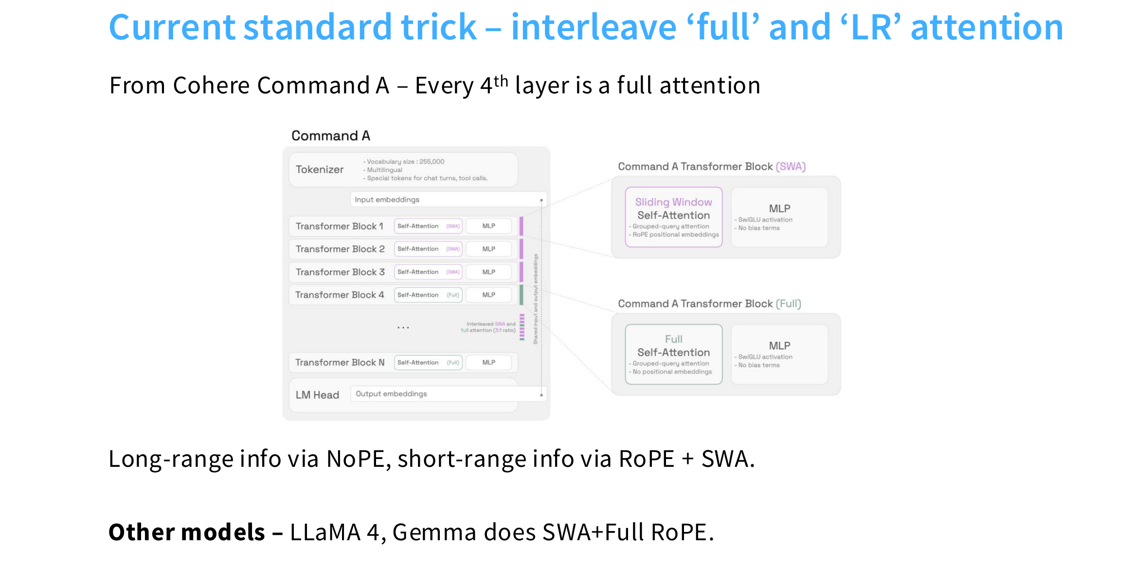
Combination

因为 Transformer 块可以实现堆叠，因此每一个堆叠的 Transformer 块可以设计不同的结构，来同时捕捉长程和短程的序列信息。

Reformer

Large Transformer models routinely achieve state-of-the-art results on a number of tasks but training these models can be prohibitively costly, especially on long sequences. We introduce two techniques to improve the efficiency of Transformers. For one, we replace dot-product attention by one that uses locality-sensitive hashing, changing its complexity from O(L2) to O(L log L), where L is the length of the sequence. Furthermore, we use reversible residual layers instead of the standard residuals, which allows storing activations only once in the training process instead of N times, where N is the number of layers. The resulting model, the Reformer, performs on par with Transformer models while being much more memory-efficient and much faster on long sequences.

A lot more about formers for lightening attention and sparse attention! We will discuss it further in the future.