LLML CS336 Lecture 2 Pytorch Resource Accounting

Source Code: Resource Accounting

Lecture 2: Pytorch & Resource Accounting

import torch

Basic Concepts

Efficiency matters!

• Compute: FLOPS

• Memory: GB

Definition of FLOPS: a metric used to measure the computational power of a computer or processor. It indicates how many floating-point operations (calculations involving decimal numbers like addition, subtraction, multiplication, and division) a system can perform per second.

$$\text{FLOPS (Ideal)} = \text{Number of Cores} \times \text{Clock Frequency per Core} \times \text{Floating Point Operations per cycle}$$

$$\text{FLOPS (Actual)} = \frac{\text{Total Number of Floating Point Operations Performed}}{\text{Execution Times}}$$

Memory Accounting

Tensors are the basic building block for storing everything: parameters, gradients, optimizer state, data, activations.

Official Docs

Almost everything (parameters, gradients, activations, optimizer states) are stored as floating point numbers.

How to compute memory bytes in Tensors?

def get_memory_usage(x: torch.Tensor):
    return x.numel() * x.element_size()

# torch.numel: Returns the total number of elements in the input tensor.
# torch.element_size: Returns the size in bytes of an individual element.

The result shows how many bytes (1 MB = $2^{20}$ bytes) a tensor is.

Basic Type

• float32: 1 + 8 + 23, default type
• float16: 1 + 5 + 10, cuts down the memory
• bfloat16: 1 + 8 + 7.
• fp8: 1 + 4 + 3 (FP8E4M3) & 1 + 5 + 2 (FP8E5M2)

Google Brain developed bfloat (brain floating point) in 2018 to address this issue. bfloat16 uses the same memory as float16 but has the same dynamic range as float32! The only catch is that the resolution is worse, but this matters less for deep learning.

FP8

Solution: use mixed precision training

def get_memory_usage(x: torch.Tensor):
    return x.numel() * x.element_size()


# torch.numel: Returns the total number of elements in the input tensor.
# torch.element_size: Returns the size in bytes of an individual element.

# for float 32
x = torch.zeros((4, 8, 20))  # @inspect x
print(x.dtype)
print("Number of elements in this tensor: ", x.numel())
print("The size of bytes for an individual element in this tensor: ", x.element_size())
print(get_memory_usage(x), "bytes")
print(get_memory_usage(x) / 2**20)

# for empty tensor?
try:
    empty_tensor = torch.empty(4, 8)
    print(get_memory_usage(empty_tensor))
except Exception as e:
    print(e)


# for float 16
x = torch.ones((4, 8, 20), dtype=torch.float16)
print(x.dtype)
print(x.numel())
print(x.element_size())
# cut the half!
print(get_memory_usage(x))

def get_bytes_information(type):
    x = torch.ones((4, 8, 20), dtype=type)
    print(f"=============={type}================")
    print(f"Dtype: {x.dtype}")
    print(f"Element size: {x.element_size()}")
    print(f"Bytes: {get_memory_usage(x)}")
    print(f"=============={type}================")
    print("\n")


TYPELIST = [torch.float64, torch.float32, torch.float, torch.float16, torch.bfloat16]

for type in TYPELIST:
    get_bytes_information(type=type)

float32_info = torch.finfo(torch.float32)  # @inspect float32_info
float16_info = torch.finfo(torch.float16)  # @inspect float16_info
bfloat16_info = torch.finfo(torch.bfloat16)  # @inspect bfloat16_info
print(float16_info)
print(float32_info)
print(bfloat16_info)

Compute Accounting

Tensors on GPU

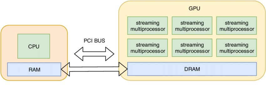
By default, tensors are stored in CPU memory. However, in order to take advantage of the massive parallelism of GPUs, we need to move them to GPU memory.

# basic information of GPUs
num_gpus = torch.cuda.device_count()  # @inspect num_gpus
for i in range(num_gpus):
    properties = torch.cuda.get_device_properties(i)  # @inspect properties
    print(properties)

print(num_gpus)

import time

x = torch.zeros((4, 8, 10))
print(x.device)

# moving the cpu to gpu
# quite slow if the tensor is large
y = x.to(device=torch.device("cuda:0"))


def test_time_compute(x: torch.Tensor):
    start_time = time.time()
    moved = x.to(device=torch.device("cuda:0"))
    print(moved.device)
    end_time = time.time()
    print(end_time - start_time)


test_time_compute(torch.zeros(size=(20, 20)))
test_time_compute(torch.zeros(size=(50000, 50000)))


# creating a tensor directly to gpu
memory_allocated = torch.cuda.memory_allocated("cuda:1")
time_1 = time.time()
z = torch.zeros(size=(50000, 50000), device="cuda:1")
time_2 = time.time()
print(time_2 - time_1)
memory_allocated_new = torch.cuda.memory_allocated(device="cuda:1")
memory_used = memory_allocated_new - memory_allocated

print(f"Memory Used: {memory_used}")

Tensor Operations

Tensor Storage

PyTorch tensors are pointers into allocated memory, with metadata describing how to get to any element of the tensor.

For the methods, we use .stride()

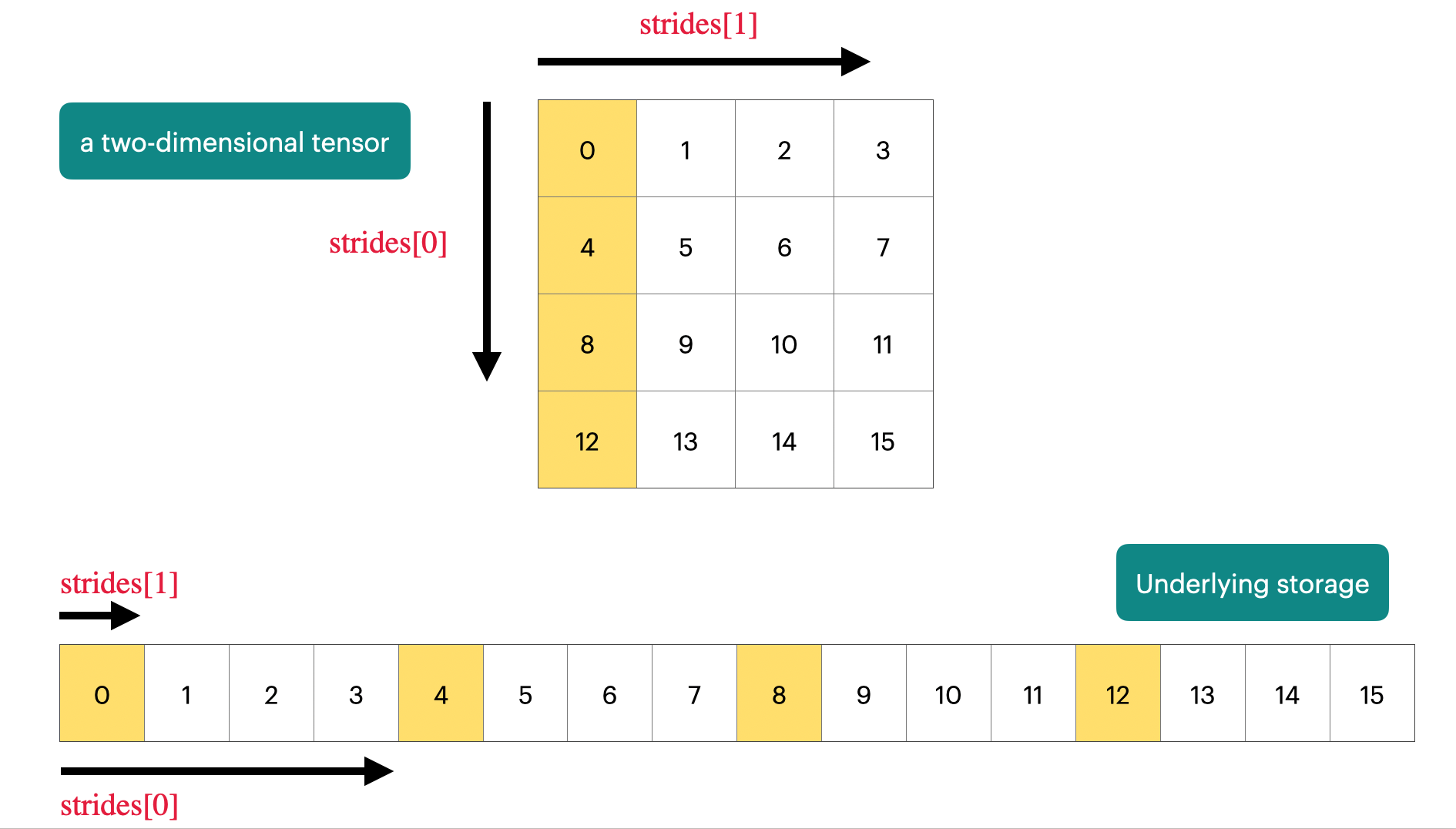
Stride is the jump necessary to go from one element to the next one in the specified dimension dim. A tuple of all strides is returned when no argument is passed in. Otherwise, an integer value is returned as the stride in the particular dimension dim.

test_tensor = torch.randint(1, 1000, size=(10, 10, 20))
print(test_tensor.shape)
print(test_tensor.dim())

# for the first dimension, it will jump 200 steps for reaching the next element
print(test_tensor.stride(0))

# for the second dimension, it will jump 20 steps for reaching the next element
print(test_tensor.stride(1))

# for the last dimension, it will jump 1 step for reaching the next element
print(test_tensor.stride(-1))

print(test_tensor[2,3,4])

How it works? For example, I want to access the value of test_tensor[i,j,k]: I will move: test_tensor.stride(0) * i + test_tensor.stride(1) * j + test_tensor.stride(2) * k.

# other operations for tensor: slicing & element_wise
# ! all the elementwise operations are operated by single element!
x = torch.Tensor([3,3,4])
print(x.pow(2))
print(x.rsqrt())

# `triu` takes the upper triangular part of a matrix.
test = torch.randint(1, 1000, size=(2, 2, 2))
print(test.triu())

Tensor Einops

Einops is a library for manipulating tensors where dimensions are named. It is inspired by Einstein summation notation (Einstein, 1916).

Official Docs

# einops demo
from einops import rearrange, reduce, repeat
from PIL import Image
from torchvision import transforms
from torchvision.transforms import ToPILImage

transform = transforms.ToTensor()
# assume there is an image called background.png
try:
    pil_image = Image.open("../../img/background.png")
    original_tensor = transform(pil_image)
except Exception as e:
    print(f"{e}")
    original_tensor = torch.randn(size=(4, 1144, 1718))

original_tensor = original_tensor[:, :1140, :1700]
print(original_tensor.shape)
# torch.Size([4, 1144, 1718]): (c, h, w)


def _to_img(my_tensor, file_path):
    if my_tensor.max() > 1.0:
        my_tensor = my_tensor / 255.0
    to_pil_image = ToPILImage()
    pil_image = to_pil_image(my_tensor)
    pil_image.save(f"../../img/{file_path}.png")


rearrange_tensor = rearrange(original_tensor, "c h w -> c w h")
_to_img(rearrange_tensor, "rearrange_background")

reduce_tensor = reduce(
    original_tensor, "c (h h2) (w w2) -> c h w", "mean", h2=20, w2=20
)
# do average pooling (like the CNN) for given tensor
print(reduce_tensor.shape)
_to_img(reduce_tensor, "reduce_background")

reduce_tensor = original_tensor[1, :, :].squeeze()
print(reduce_tensor.shape)
repeat_tensor = repeat(reduce_tensor, "h w -> c h w", c=4)
_to_img(repeat_tensor, "repeat_background")

JaxTyping

jaxtyping is a Python library that provides type annotations for your array-based code, particularly for the JAX framework. Think of it as a tool that lets you add precise shape and data type information to your function signatures, going far beyond the basic jax.Array or np.ndarray type hints.

For torch.Tensor, things get the same.

Moreover, jax support JIT and auto-grad functions.

from jaxtyping import Float
x: Float[torch.Tensor, "batch seq heads hidden"] = torch.ones(2, 2, 1, 3)  # @inspect x

print(x)

import jax
from jax import numpy as jnp
from jaxtyping import Float, Int

def matmul(
    A: Float[jax.Array, "batch_size in_features"],
    B: Float[jax.Array, "in_features out_features"]
) -> Float[jax.Array, "batch_size out_features"]:
    """Performs matrix multiplication."""
    return A @ B

# This will pass type checking
A_good = jnp.zeros((128, 784))
B_good = jnp.zeros((784, 10))
result = matmul(A_good, B_good)
print(result.shape) # (128, 10)

# A static type checker will flag an error here because "in_features"
# dimensions don't match (784 vs 600).
A_bad = jnp.zeros((128, 784))
B_bad = jnp.zeros((600, 10))
# result = matmul(A_bad, B_bad)

einsum

By using einops, we can run this code in a better way!

from jaxtyping import Float
from einops import einsum

B = 128
SEQ1 = 100
SEQ2 = 200
HIDDEN_DIM = 128

x: Float[torch.Tensor, "batch seq1 hidden_dim"] = torch.randn(size=(B, SEQ1, HIDDEN_DIM))
y: Float[torch.Tensor, "batch seq2 hidden_dim"] = torch.randn(size=(B, SEQ2, HIDDEN_DIM))

z = einsum(x, y, "batch seq1 hidden_dim, batch seq2 hidden_dim -> batch seq1 seq2")
print(x.shape)
print(y.shape)
print(torch.equal(z, (x @ y.transpose(-2, -1))))
print(z.shape)

reduce

You can reduce a single tensor via some operation (e.g., sum, mean, max, min).

x: Float[torch.Tensor, "batch seq hidden"] = torch.ones(2, 3, 4)  # @inspect x
# Old way:
y = x.mean(dim=-1)  # @inspect y
# New (einops) way:
y = reduce(x, "... hidden -> ...", "sum")  # @inspect y

x: Float[torch.Tensor, "batch seq hidden"] = torch.randn(2, 3, 4)  # @inspect x

# make the last dimension mean to 0
x = x - torch.mean(x, dim=-1, keepdim=True)

y = reduce(x, "... hidden -> ...", "sum")  # @inspect y
print(y.shape)
print(y)

rearrange

Sometimes, a dimension represents two dimensions.

x: Float[torch.Tensor, "batch seq total_hidden"] = torch.ones(2, 3, 8)  # @inspect x
# ...where total_hidden is a flattened representation of heads * hidden1
w: Float[torch.Tensor, "hidden1 hidden2"] = torch.ones(4, 2)

print(f"x shape: {x.shape}")

# Break up total_hidden into two dimensions (heads and hidden1):
# total_hidden = hidden1 \times hidden2
x = rearrange(x, "... (heads hidden1) -> ... heads hidden1", heads=2)  # @inspect x
print(f"x shape: {x.shape}")

# Perform the transformation by w:
x = einsum(x, w, "... hidden1, hidden1 hidden2 -> ... hidden2")  # @inspect x
# Combine heads and hidden2 back together:
print(f"x shape: {x.shape}")
x = rearrange(x, "... heads hidden2 -> ... (heads hidden2)")  # @inspect x
print(f"x shape: {x.shape}")

Computation Cost

Having gone through all the operations, let us examine their computational cost.

A floating-point operation (FLOP) is a basic operation like addition (x + y) or multiplication (x y).

• FLOPs: floating-point operations (measure of computation done)
• FLOP/s: floating-point operations per second (also written as FLOPS), which is used to measure the speed of hardware.

Several Statistics

• GPT-3: 3.14e23 FLOPs

• GPT-4: 2e25 FLOPS

• A100 has a peak performance of 312 teraFLOP/s. (teraFLOPS = 1e12 FLOPS)

  • 17806267 hours (total)

linear model demo

Core: Matrix Multiplications

if torch.cuda.is_available():
    B = 16384  # Number of points
    D = 32768  # Dimension
    K = 8192   # Number of outputs
else:
    B = 1024
    D = 256
    K = 64
device = "cuda" if torch.cuda.is_available() else "cpu"
x = torch.ones(B, D, device=device)
w = torch.randn(D, K, device=device)
y = x @ w
# We have one multiplication (x[i][j] * w[j][k]) and one addition per (i, j, k) triple.
actual_num_flops = 2 * B * D * K  # @inspect actual_num_flops

print(actual_num_flops)

Interpretation:

• B is the number of data points

• (D K) is the number of parameters

FLOPs for forward pass is 2 (# tokens) (# parameters)

It turns out this generalizes to Transformers (to a first-order approximation).

Model FLOPS Utilization

$\text{MFU} = \frac{\text{actual FLOPS}}{\text{promised FLOPS}}$

• $\text{actual FLOPS} = \frac{\text{sum FLOPs}}{\text{time}}$

• $\text{promised FLOPS}$ is provided by the hardware company.

Usually, MFU of >= 0.5 is quite good (and will be higher if matmuls dominate)

Time Complexity for Several Operations

Consider Matrix $A$: $(m,n)$ and matrix $B$: $(n,k)$.

• FLOPs for matrix multiplications: $m \times n \times (2k)$

• Elementwise operation on a $m \times n$ matrix requires $O(m n)$ FLOPs.

• Addition of two $m \times n$ matrices requires $m n$ FLOPs.

FLOPs depends highly on hardware and data types.

Gradient Basics

Computing Gradients also need computation resources!

Consider simple linear regression model:

x = torch.tensor([1., 2, 3])
w = torch.tensor([1., 1, 1], requires_grad=True)  # Want gradient
pred_y = x @ w
loss = 0.5 * (pred_y - 5).pow(2)

Let’s get some Math:

$$L(\vec{w}) = \frac{1}{2}(\vec{x} \cdot \vec{w} - y_{\text{true}})^2$$

$$\nabla f = \frac{\partial L}{\partial \vec{w}} = (\frac{\partial L}{\partial w_1}, \frac{\partial L}{\partial w_2}, \frac{\partial L}{\partial w_3}) = (\vec{x} \cdot \vec{w} - y_{\text{true}}) · (x_1, x_2, x_3)$$

x = torch.tensor([1., 2, 3])
w = torch.tensor([1., 1, 1], requires_grad=True)  # Want gradient

# do doct product
pred_y = x @ w

# MSE Error
loss = 0.5 * (pred_y - 5).pow(2)

print(x.shape)
print(w.shape)
print(loss)


# run loss backward
loss.backward()
print(w.grad)

Gradient Flops

Forward Pass

Just the simple matrix multiplications.

For the neural network, we can make things more complex.

import torch
if torch.cuda.is_available():
    B = 16384  # Number of points
    D = 32768  # Dimension
    K = 8192   # Number of outputs
else:
    B = 1024
    D = 256
    K = 64
device = "cuda" if torch.cuda.is_available() else "cpu"
x = torch.ones(B, D, device=device)
w1 = torch.randn(D, D, device=device, requires_grad=True)
w2 = torch.randn(D, K, device=device, requires_grad=True)
# Model: x --w1--> h1 --w2--> h2 -> loss
h1 = x @ w1
print(h1.shape) # (B, D)
h2 = h1 @ w2
loss = h2.pow(2).mean()

# FLOPs
# two layers, thus two matrix multiplications
num_forward_flops = (2 * B * D * D) + (2 * B * D * K)

torch.Size([16384, 32768])

print(f"{num_forward_flops:.3e}")
print(loss.shape)
print(h2.shape)

h1.retain_grad()
h2.retain_grad()
loss.backward()

4.398e+13
torch.Size([])
torch.Size([16384, 8192])

Backward Pass

Several computation for gradients.

# x = torch.ones(B, D, device=device)
# w1 = torch.randn(D, D, device=device, requires_grad=True)
# w2 = torch.randn(D, K, device=device, requires_grad=True)
# # Model: x --w1--> h1 --w2--> h2 -> loss
# h1 = x @ w1
# print(h1.shape) # (B, D)
# h2 = h1 @ w2
# loss = h2.pow(2).mean()

# x: [B, D]
# w1: [D, D]
# w2: [D, K]
# h1: [B, D]
# h2: [B, K]
# loss: \in R

Forward Pass: $x \to \text{w1} \to \text{h1} \to \text{w2} \to \text{h2} \to \text{loss}$

Backward Pass: Starting from the loss, the gradient of each parameter is calculated in reverse.

The gradient calculation follows the chain rule:

$$\frac{\partial \text{loss}}{\partial w_{2,jk}} = \sum_{i} \frac{\partial \text{loss}}{\partial h_{2,ik}} \cdot \frac{\partial h_{2,ik}}{\partial w_{2,jk}}$$

• $\frac{\partial \text{loss}}{\partial w_{2,jk}}$ is the gradient of the $(j, k)$ element of w2 that we want to calculate.
• $h_{2,ik}$ is the $(i, k)$ element of h2.
• $\frac{\partial \text{loss}}{\partial h_{2,ik}}$ is the gradient of the $(i, k)$ element of h2 (i.e., h2.grad[i,k]).
• We need to sum over all relevant intermediate variables, which in this case are all rows i of h2.

It is the element-wise format of:

$$\frac{\partial \text{loss}}{\partial \mathbf{w}_2} = \frac{\partial \text{loss}}{\partial \mathbf{h}_2} \cdot \frac{\partial \mathbf{h}_2}{\partial \mathbf{w}_2}$$

h2 is obtained through the matrix multiplication of h1 and w2.The $(i, k)$ element of h2, $h_{2,ik}$, is calculated as:

$$h_{2,ik} = \sum_{t=1}^{p} h_{1,it} \cdot w_{2,tk}$$

Now, we calculate the partial derivative of $h_{2,ik}$ with respect to $w_{2,jk}$.

$$\frac{\partial h_{2,ik}}{\partial w_{2,jk}} = \frac{\partial}{\partial w_{2,jk}} \left( \sum_{t=1}^{p} h_{1,it} \cdot w_{2,tk} \right) = h_{1, ij}$$

Substituting our derived $\frac{\partial h_{2,ik}}{\partial w_{2,jk}} = h_{1,ij}$ into the chain rule formula:

$$\frac{\partial \text{loss}}{\partial w_{2,jk}} = \sum_{i} \frac{\partial \text{loss}}{\partial h_{2,ik}} \cdot h_{1,ij}$$

Representing this formula using PyTorch terminology, we get the content from the image:

$$\text{w2.grad}[j,k] = \sum_{i} \text{h2.grad}[i,k] \cdot \text{h1}[i,j]$$

For the matrix format:

$$\mathbf{w}_2.\text{grad} = \mathbf{h}_1^{\top} \cdot \mathbf{h}_2.\text{grad}$$

Time cost?

print(w2.grad.size()) # (D, K)
print(h1.size()) # (B, D)
print(h2.grad.size()) # (B, K)

Still a matrix multiplication! Time: $2B \times D \times K$.

For the similar algorithms for $\mathbf{w}_1$, things remain the same.

$$\frac{\partial \text{loss}}{\partial \text{h1}} = \frac{\partial \text{loss}}{\partial \text{h2}} \cdot \frac{\partial \text{h2}}{\partial \text{h1}}$$

$$\text{h1.grad} = \text{h2.grad} \cdot \text{w2}^\mathsf{T}$$

$$\text{w1.grad} = \text{x}^\mathsf{T} \cdot \text{h1.grad}$$

$$\text{x.grad} = \mathbf{h}_1.\text{grad} \cdot \mathbf{w}_1^{\top}$$

• Compute h1.grad: $2BDK$
• Compute w1.grad: $2BD^2$
• Compute x.grad: $2BD^2$ (actually unnecessary)

Sum for Backward Pass: $4 \times B \times (D^2 + DK)$

print(w2.size())
print(w2.grad.size()) # (D, K)

print(h1.size()) # (B, D)
print(h1.grad.size()) # (B, D)

print(h2.grad.size()) # (B, K)
print(h2.size())

print(w1.size()) # (D, D)

torch.Size([32768, 8192])
torch.Size([32768, 8192])
torch.Size([16384, 32768])
torch.Size([16384, 32768])
torch.Size([16384, 8192])
torch.Size([16384, 8192])
torch.Size([32768, 32768])

Putting it togther:

( # parameters) = the number of all the parameters, which is $w_1$ and $w_2$ in this model ($ D \times D + D \times K$).

• Forward pass: 2 (# data points) (# parameters) FLOPs = $2B(D^2 + DK)$

• Backward pass: 4 (# data points) (# parameters) FLOPs = $4B(D^2 + DK)$

• Total: 6 (# data points) (# parameters) FLOPs

Thus:

Question: How long would it take to train a 70B parameter model on 15T tokens on 1024 H100s? total_flops = 6 * 70e9 * 15e12 # @inspect total_flops

Models

Module Parameters

Initialization

When the input dimension input_dim of a neural network layer is large, its output values also tend to become very large.

For example, output = x @ w describes a multiplication of a vector x by a weight matrix w. If the elements of both x and w are sampled randomly from a standard normal distribution, then according to probability theory, the variance of each element in the output output is proportional to input_dim.

For example, the $j$-th element of output is:

$$\text{output}_j = \sum_{i=1}^{\text{input\_dim}} x_i \cdot w_{ij}$$

If $x_i$ and $w_{ij}$ have a mean of 0 and a variance of 1, then the variance of $\text{output}_j$ is:

$$\text{Var}(\text{output}_j) = \sum_{i=1}^{\text{input\_dim}} \text{Var}(x_i \cdot w_{ij})$$

$$= \sum_{i=1}^{\text{input\_dim}} \text{Var}(x_i) \cdot \text{Var}(w_{ij}) = \text{input\_dim} \cdot 1 \cdot 1 = \text{input\_dim}$$

This means the standard deviation of output is $\sqrt{\text{input\_dim}}$. This could cause damages when the input dim scales larger, for instance: gradient vanishing, etc.

Xavier Initialization

Data Loader

In language modeling, data is a sequence of integers (output by the tokenizer). It is convenient to serialize them as numpy arrays (done by the tokenizer).

orig_data = np.array([1, 2, 3, 4, 5, 6, 7, 8, 9, 10], dtype=np.int32)
orig_data.tofile("data.npy")
# You can load them back as numpy arrays.
# Don't want to load the entire data into memory at once (LLaMA data is 2.8TB).
# Use memmap to lazily load only the accessed parts into memory.
data = np.memmap("data.npy", dtype=np.int32)
assert np.array_equal(data, orig_data)
# A data loader generates a batch of sequences for training.
B = 2  # Batch size
L = 4  # Length of sequence
x = get_batch(data, batch_size=B, sequence_length=L, device=get_device())
assert x.size() == torch.Size([B, L])

Optimizer

Let’s define the AdaGrad optimizer

• momentum = SGD + exponential averaging of grad

• AdaGrad = SGD + averaging by grad^2

• RMSProp = AdaGrad + exponentially averaging of grad^2

• Adam = RMSProp + momentum

SGD (Stochastic Gradient Descent)

This is the most basic optimization method. It updates model parameters by calculating the gradient of the loss function and moving in the opposite direction of the gradient.

$$w_{t+1} = w_t - \eta \cdot g_t$$

Where:

• $w_t$ is the parameter at the current time step.
• $\eta$ is the learning rate, a hyperparameter that controls the step size.
• $g_t$ is the gradient at the current time step.

Main Problem: The learning rate is fixed. This can cause the optimizer to move too fast in steep areas and too slow in flat areas. It also tends to oscillate in certain directions.

AdaGrad (Adaptive Gradient Algorithm)

AdaGrad is an improvement over SGD that introduces the concept of an adaptive learning rate. It uses a different learning rate for each parameter, and these rates decay over time during training.

Core Idea: It scales the learning rate for each parameter by accumulating the sum of the squares of all past gradients.

$$G_t = \sum_{\tau=1}^{t} g_{\tau}^2$$

$$w_{t+1} = w_t - \frac{\eta}{\sqrt{G_t + \epsilon}} \cdot g_t$$

Where:

• $G_t$ is the sum of the squared gradients from the start of training up to the current time step.
• $\epsilon$ is a small constant to prevent division by zero.

Advantage: It’s well-suited for sparse data, as parameters that are updated infrequently get a larger learning rate.

Main Problem: Since $G_t$ is a monotonically increasing sum, the learning rate for all parameters will eventually become extremely small, halting further learning in the later stages of training.

RMSProp (Root Mean Square Propagation)

RMSProp addresses the issue of AdaGrad’s rapidly decaying learning rate. Instead of accumulating the sum of all past squared gradients, it uses an exponentially weighted moving average of the squared gradients. This allows it to “forget” distant past gradients, preventing the learning rate from decaying too quickly.

Core Idea: It replaces AdaGrad’s cumulative sum with an exponential moving average.

$$E[g^2]_t = \gamma \cdot E[g^2]_{t-1} + (1-\gamma) \cdot g_t^2$$

$$w_{t+1} = w_t - \frac{\eta}{\sqrt{E[g^2]_t + \epsilon}} \cdot g_t$$

Where:

• $E[g^2]_t$ is the exponentially weighted moving average of the squared gradients.
• $\gamma$ is a decay rate, typically set to 0.9 or 0.99.

Advantage: It solves the premature learning rate decay problem of AdaGrad, allowing the model to continue learning throughout training.

Adam (Adaptive Moment Estimation)

Adam combines the best of RMSProp and Momentum. It maintains an exponentially weighted moving average of both the gradients (the momentum term) and the squared gradients (the RMSProp term).

Core Idea:

• First moment: An exponentially weighted moving average of the gradients (the momentum term).

$$m_t = \beta_1 m_{t-1} + (1-\beta_1) g_t$$

• Second moment: An exponentially weighted moving average of the squared gradients (the RMSProp term).

$$v_t = \beta_2 v_{t-1} + (1-\beta_2) g_t^2$$

$$v_{t}=\left(1-\beta_{2}\right) \sum_{i=1}^{t} \beta_{2}^{t-i} g_{i}^{2}$$

v represents variance. $\text{Var}(g) = \mathbb{E}[g^2] - (\mathbb{E}[g])^2$, and $v_t$ represents the moving average squared gradients. Thus we have: $\text{Var}(g) \approx v_t - (m_t)^2$ $v_t$ and $m_t$ are all moving average of $g^2$ and $g$, which in essence is a weighted average.

• Adam also includes a bias correction, as $m_t$ and $v_t$ are biased towards zero in the initial training steps.
• The final update rule after bias correction is:

$$\hat{m}_t = \frac{m_t}{1-\beta_1^t}, \quad \hat{v}_t = \frac{v_t}{1-\beta_2^t}$$

$$w_{t+1} = w_t - \frac{\eta}{\sqrt{\hat{v}_t} + \epsilon} \cdot \hat{m}_t$$

Advantage: It combines the benefits of momentum and adaptive learning rates, leading to faster convergence and often superior performance. Adam is a highly popular and widely used optimizer for a wide range of deep learning tasks.

Memory

# Parameters
num_parameters = (D * D * num_layers) + D  # @inspect num_parameters
assert num_parameters == get_num_parameters(model)
# Activations
num_activations = B * D * num_layers  # @inspect num_activations
# Gradients
num_gradients = num_parameters  # @inspect num_gradients
# Optimizer states
num_optimizer_states = num_parameters  # @inspect num_optimizer_states
# For Adam, it is 2 * num_parameters

# Putting it all together, assuming float32
total_memory = 4 * (num_parameters + num_activations + num_gradients + num_optimizer_states)  # @inspect total_memory

Checkpoint

Training language models take a long time and will certainly crash. You don’t want to lose all your progress. During training, it is useful to periodically save your model and optimizer state to disk.

model = Cruncher(dim=64, num_layers=3).to(get_device())
optimizer = AdaGrad(model.parameters(), lr=0.01)
# Save the checkpoint:
checkpoint = {
    "model": model.state_dict(),
    "optimizer": optimizer.state_dict(),
}
torch.save(checkpoint, "model_checkpoint.pt")
# Load the checkpoint:
loaded_checkpoint = torch.load("model_checkpoint.pt")

Mixed Precision Training

Choice of data type (float32, bfloat16, fp8) have tradeoffs.

• Higher precision: more accurate/stable, more memory, more compute

• Lower precision: less accurate/stable, less memory, less compute

Solution: use float32 by default, but use {bfloat16, fp8} when possible. A concrete plan:

• Use {bfloat16, fp8} for the forward pass (activations).

• Use float32 for the rest (parameters, gradients).

Pytorch has an automatic mixed precision (AMP) library.

• https://pytorch.org/docs/stable/amp.html
• https://docs.nvidia.com/deeplearning/performance/mixed-precision-training/

Transformers for Resource Accounting

• Transformer Memory

• Transformer FLOPs