My final assignment for Introduction to artificial intelligence.
Tracing the Evolution of ILSVRC Winners and Their Impact on Image Classifications
Abstract
The past decade witnessed the transformation from Fully Connected Neural Network(FCNN) to Convolutional Neural Network(CNN) , which significantly addressed various challenges in the field of image recognition. This review traces how deep learning had passed a decade of breakthrough, introducing the evolution of winners from the ImageNet Large Scale Visual Recognition Challenge (ILSVRC), highlighting key advancements such as AlexNet, GoogLeNet, ResNet and ResNeXt. By analyzing the architectural innovations and methodological breakthroughs of these models such as ReLU, dropout, LRN, Inception, Residual Network and cardinality, the review then provides insights into the trends in neural network research, regarding how they implemented the optimization by adding the depth of the layers without introducing a huge amount of extra parameters and computational complexity. Finally, we discussed the outlook of Deep Neural Networks in the field of image classification, including striving for higher quality datasets, moving from object recognition to human-level understanding and finding alternative models outperforming traditional CNNs.
""" Author: Xiyuan Yang xiyuan_yang@outlook.com Date: 2025-04-14 19:23:55 LastEditors: Xiyuan Yang xiyuan_yang@outlook.com LastEditTime: 2025-04-14 19:24:01 FilePath: /CNN-tutorial/src/convolution.py Description: Do you code and make progress today? Copyright (c) 2025 by Xiyuan Yang, All Rights Reserved. """
import numpy as np import matplotlib.pyplot as plt import matplotlib as mlp from scipy.integrate import quad
mlp.use("Agg")
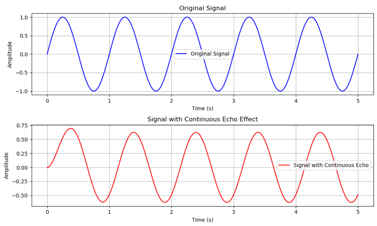
# Original Function f(t) deforiginal_signal(t): return np.sin(2 * np.pi * t)
defecho_kernel2(t, alpha): if t >= 0: return np.exp(-alpha * t) else: return0.0
# Normalize the kernel to ensure its integral is 1 defnormalized_echo_kernel(t, alpha): # Compute the normalization factor (integral of the kernel from 0 to infinity) normalization_factor, _ = quad(lambda tau: echo_kernel2(tau, alpha), 0, np.inf) # Return the normalized kernel value return echo_kernel2(t, alpha) / normalization_factor
# Convolution with normalized kernel defconvolution(f, g, t_values, alpha): h = [] for t in t_values: integral, _ = quad(lambda tau: f(tau) * g(t - tau, alpha), 0, t) h.append(integral) return np.array(h)
# Plot figure for two pictures defplotfig(t, f, h, alpha): plt.figure(figsize=(10, 6))
# Original Signal plt.subplot(2, 1, 1) plt.plot(t, f, label="Original Signal", color="blue") plt.title("Original Signal") plt.xlabel("Time (s)") plt.ylabel("Amplitude") plt.legend() plt.grid()
# Signal with Continuous Echo Effect plt.subplot(2, 1, 2) plt.plot(t, h, label="Signal with Continuous Echo", color="red") plt.title("Signal with Continuous Echo Effect") plt.xlabel("Time (s)") plt.ylabel("Amplitude") plt.legend() plt.grid() plt.tight_layout() plt.savefig(f"img/Signal_with_Continuous_Effect_alpha={alpha:.2f}.png") plt.close()
defmain(): t = np.linspace(0, 5, 500) # Time range from 0 to 5 seconds f = original_signal(t) # Original signal
# Test different values of alpha for i in [0.01, 0.1, 0.3, 0.5, 0.6, 0.8, 1, 1.1, 1.4, 1.5, 2, 2.5, 5]: h = convolution(original_signal, normalized_echo_kernel, t, alpha=i) plotfig(t, f, h, i)
""" Author: Xiyuan Yang xiyuan_yang@outlook.com Date: 2025-04-15 00:28:15 LastEditors: Xiyuan Yang xiyuan_yang@outlook.com LastEditTime: 2025-04-15 00:29:55 FilePath: /CNN-tutorial/src/convolution_demo.py Description: Do you code and make progress today? Copyright (c) 2025 by Xiyuan Yang, All Rights Reserved. """
import torch import torch.nn.functional as F from PIL import Image import torchvision.transforms as transforms import matplotlib.pyplot as plt import matplotlib as mlp import numpy as np
""" Author: Xiyuan Yang xiyuan_yang@outlook.com Date: 2025-04-15 14:40:20 LastEditors: Xiyuan Yang xiyuan_yang@outlook.com LastEditTime: 2025-04-15 14:41:31 FilePath: /CNN-tutorial/src/AlexNet.py Description: Do you code and make progress today? Copyright (c) 2025 by Xiyuan Yang, All Rights Reserved. """
import torch import torch.nn as nn import torch.nn.functional as F
defforward(self, x): # Pass input through the convolutional layers x = self.features(x)
# Flatten the output for the fully connected layers x = torch.flatten(x, 1)
# Pass through the fully connected layers x = self.classifier(x) return x
# Example usage if __name__ == "__main__": # Create an instance of AlexNet with 1000 output classes (default for ImageNet) model = AlexNet(num_classes=1000)
# Print the model architecture print(model)
# Test with a random input tensor (batch size 1, 3 channels, 224x224 image) input_tensor = torch.randn(1, 3, 224, 224) output = model(input_tensor) print(output.shape) # Should output torch.Size([1, 1000])
print("Train the Basic Alexnet: session BEGIN") import torch import torch.nn as nn import torch.optim as optim from torch.utils.data import DataLoader from torchvision import datasets, transforms from AlexNet import AlexNet
# Check if GPU is available device = torch.device("cuda"if torch.cuda.is_available() else"cpu")
defforward(self, x): x = self.features(x) x = torch.flatten(x, 1) x = self.classifier(x) return x
Something Else
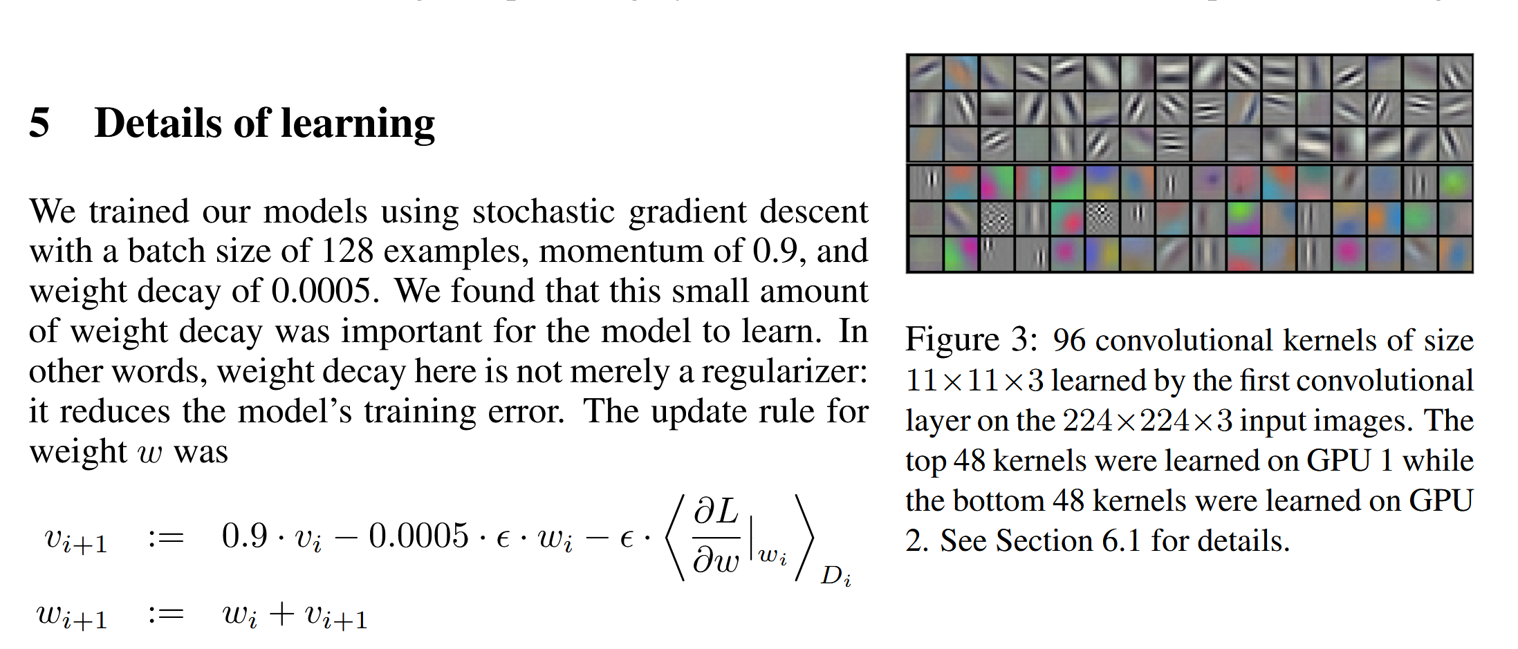
我们不妨问这样一个问题,在AlexNet的学习过程中,模型学习到了什么?
来看论文原文,Ilya是这样写的:
Figure 3 shows the convolutional kernels learned by the network’s two data-connected layers. The network has learned a variety of frequency and orientation-selective kernels, as well as various colored blobs. Notice the specialization exhibited by the two GPUs, a result of the restricted connectivity described in Section 3.5. The kernels on GPU 1 are largely color-agnostic, while the kernels on on GPU 2 are largely color-specific. This kind of specialization occurs during every run and is independent of any particular random weight initialization (modulo a renumbering of the GPUs).