DataStructure Graph SSSP Problem

SSSP Problems for unweighted graphs

We still focus on SSSP problems: single source shortest path. (We focus on directed graphs)

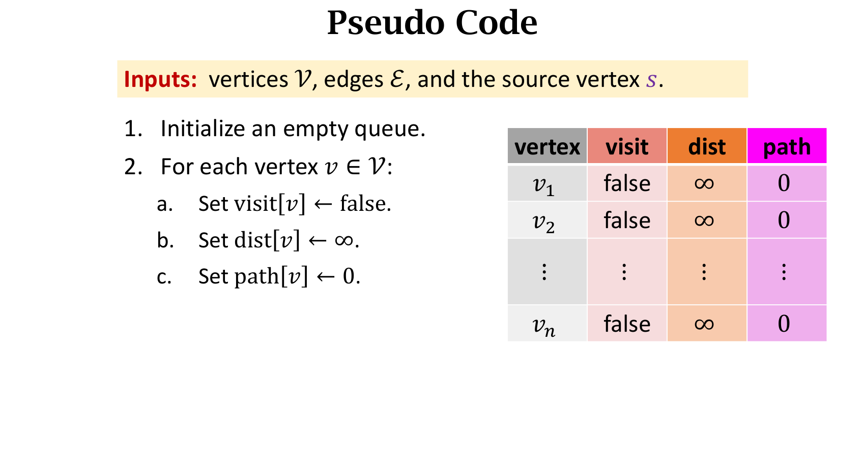
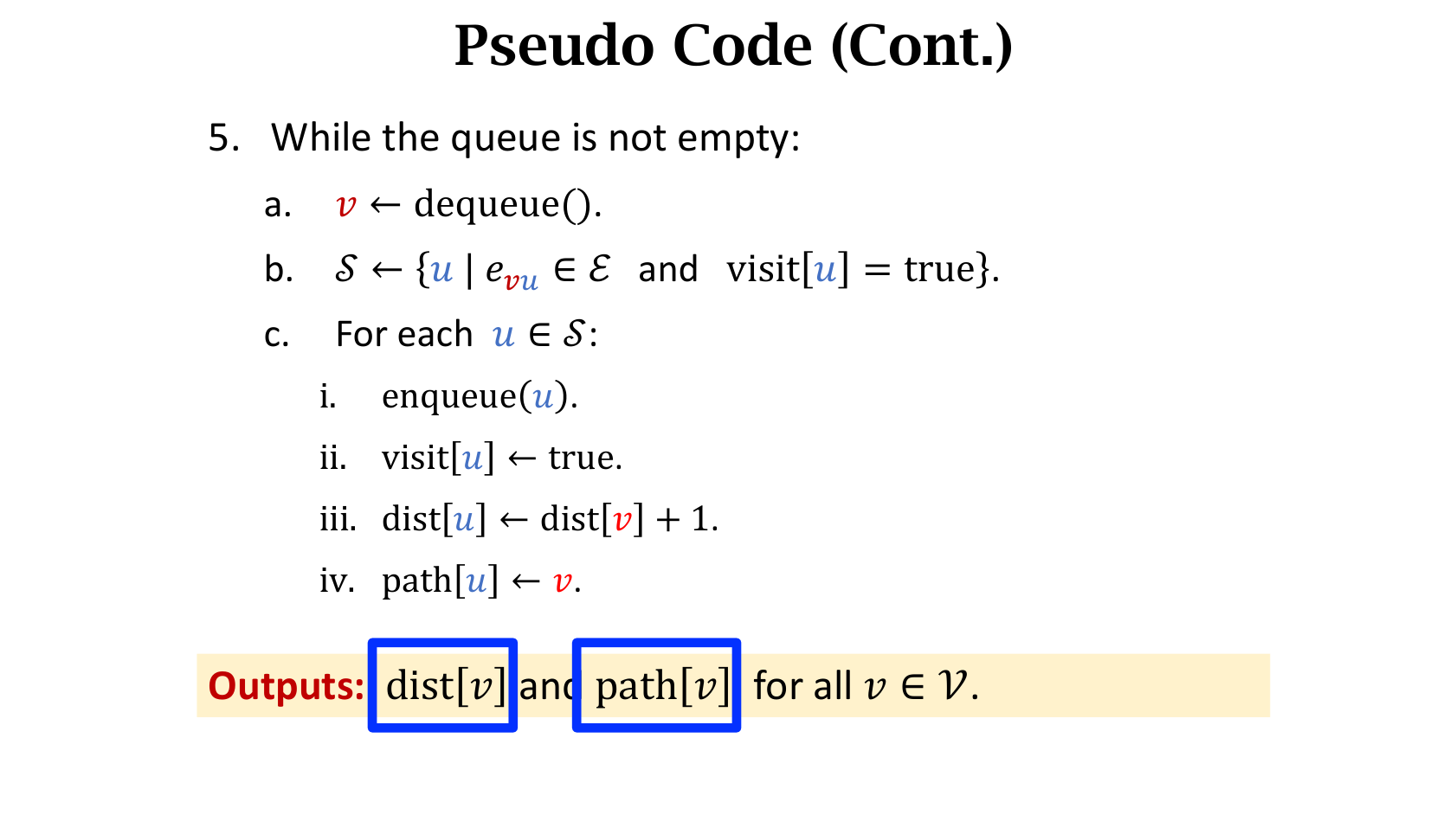
We will use BFS algorithm and Dynamic Programming to dynamically update the value from the beginning.

maintain a queue for BFS:
- Attention: this queue holds the increasing order for the distance from the single source vertex $w$.
- Hence, for every vertex, the first time it appears in the queue is the shortest path to the source vertex $w$.

You can see this video for more information

During the updating process, you can recording the information of its adjacency for the single path. Hence, despite the SSSP problems, we can still know how to go to the source via the found shortest path.

Pseudo Code

The Slides are from: https://github.com/wangshusen/AdvancedAlgorithms, really a great course for learning data structures!

Time Complexity

Time complexity:

Initialization: $O(|V|)$
Queue Operations: $O(|V|)$
- Every vertex will be euqueued and dequeued only once.
Every Edge will be visited only once: $O(|E|)$.

Hence, the time complexity is $O(|V| + |E|)$.

SSSP Problems for weighted graphs

Especially for Weighted Shorted Path Problem

For unweighted shorted path problems, we can simply use BFS algorithms to solve it!

Lecture Note for MIT 6.006

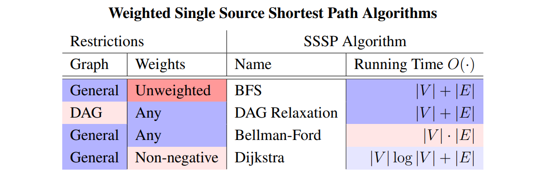
We will introduce several algorithms:

Previously

DFS & BFS problems:

Single Source Shortest Path: $O(|V| + |E|)$
Single Source Reachability: $O(|E|)$
Connected components: $O(|V| + |E|)$
Topological Sort: $O(|V| + |E|)$

Weighted Graph

For weighted graph, each edge has a weight. (Full of applications)

How to store weights:

with each adjacency, store a weight. Given a node $u$, for every adjacency $v$, stores a weight!
Set data structure: $E \to W$.

Weighted Path: $w(\pi) = \sum_{e \in \pi}w(e)$. We need to find the shortest path from given vertices $u$ to $v$.

$$\delta(u,v) = \inf\{ w(\pi)| \pi: u \to v \}$$

(if no path, define $\delta(u,v) = \infty$)

Some problems occurred! Especially when there are some circle paths and the weight of the circle path is negative! Then due to the definition, $w(\pi)$ should be $-\infty$.

Negative Weight Cycles: Not good!

For the shortest path algorithms: we can use simple BFS algorithms: Expand an weighted edge to several simple edges from $u$ to $v$. (Then we can count the shortest path by the definition of the number of the edges.): Use BFS to solve this shortest-path problems!

Disadvantages: It is linear time, needs quite large memory expansion if the weight is quite large.

Proofs

Thm: For weighted shortest path, only need parent of $v$ ($P(v)$) for $v$ only finite $\delta(u,v)$

Init: P is empty, $P(s)$ is None.
For each $u \in V$, where $\delta(s,u)$ is finite:
- For each $v \in \text{Adj}^+(u)$:
  - if $v$ not $\in P$ and $\delta(s,u) = \delta(s, v) + w(u,v)$. (Suppose it is the shortest path!)
  - $\exists w, (u,v) \in w$ and $w$ can be the shortest path. So set $P(v) = u$.

$P$ is used to construct one of the existing shortest path.

DAG

有向无环图（DAG, Directed Acyclic Graph）

It can handle with negative weights, but it cannot handle with Negative Weight Cycles.

Relaxation

For edges $(u,v)$, we need to check it is possible to shorten the shortest path from $u$ to $v$.

Obviously, we have:

$$\delta(u,v) \le \delta(u,w) + \delta(w,v)$$

Hence, if $d(s,v) > d(s,u) + w(u,v)$, then we can update $d(s,v) = d(s,u) + w(u,v)$

It is DP Problems! Because we can assert that there is no loop in the DAGs, hence we use Topological Order to ensure all the nodes are sorted in sequence.

Assume $u$ is ahead in the topological order of $v$, then $\delta(s,u)$ is computed before the $\delta(s,v)$.

For the first vertex is $s$ itself, init $d(s,s) = 0$, and $d(s,u) = \infty, u \ne s$.

In topological order, we update $d(s,v)$ by using the adjacency $u$ ,(which is computed previously) of $d(s,u) + w(u,v)$.

Then we update the optimization! Finally, $\delta(s,u) = d(s,u)$.

Time complexity: $O(|V| + |E|)$

Topo sort: $O(|V| + |E|)$
relaxation: $O(|E|)$

DAG is efficiency in SSSP! For it is based on dynamic programming. But it should ensure it is DAG! (Needs topo sort first).

Code

#include <climits>// For INT_MAX
#include <iostream>
#include <queue>
#include <unordered_map>
#include <vector>

using namespace std;

class DAG {
private:
    unordered_map<int, vector<pair<int, int>>> adj;// Adjacency list with weights
    unordered_map<int, int> inDegree;              // In-degree count, used for topologicalSorting
    int vertex_num;

public:
    DAG(int num = 0) {
        vertex_num = num;
    }

    // Add a directed edge u -> v with weight w
    void addEdge(int u, int v, int weight) {
        adj[u].emplace_back(v, weight);
        inDegree[v]++;// Increment in-degree of v
    }

    // Perform topological sort using Kahn's algorithm
    vector<int> topologicalSort() {
        vector<int> result;
        queue<int> q;

        // Initialize queue with nodes having 0 in-degree
        for (auto node : adj) {
            int u = node.first;
            if (inDegree[u] == 0) {
                q.push(u);
            }
        }

        while (!q.empty()) {
            int u = q.front();
            q.pop();
            result.push_back(u);

            // Reduce in-degree of neighbors
            for (auto &neighbor : adj[u]) {
                int v = neighbor.first;
                inDegree[v]--;
                if (inDegree[v] == 0) {
                    q.push(v);
                }
            }
        }

        cout << adj.size();
        cout << result.size();
        // Check for cycles (if result size != number of nodes)
        cout << "a" << (result.size());
        if (result.size() != adj.size()) {
            cout << "Cycle detected! Not a DAG." << endl;
            return {};
        }

        return result;
    }

    // DAG Relaxation for Single Source Shortest Path (SSSP)
    vector<int> dagRelaxation(int source) {
        // Perform topological sort
        vector<int> sortedOrder = topologicalSort();
        if (sortedOrder.empty()) {
            cout << "Cannot perform DAG relaxation due to cycle." << endl;
            return {};
        }
        vector<int> dist(vertex_num + 1, INT_MAX);// Initialize distances to infinity
        dist[source] = 0;                     // Distance to source is 0


        // Relax edges in topological order
        for (int u : sortedOrder) {
            if (dist[u] == INT_MAX) {
                continue;
            }
            for (auto &neighbor : adj[u]) {
                int v = neighbor.first;
                int weight = neighbor.second;
                // update
                if (dist[u] + weight < dist[v]) {
                    dist[v] = dist[u] + weight;
                }
            }
        }
        return dist;
    }
};

int main() {
    DAG dag(5);

    // Build a sample DAG with weights
    dag.addEdge(1, 2, 3);// Edge 1 -> 2 with weight 3
    dag.addEdge(1, 3, 6);// Edge 1 -> 3 with weight 6
    dag.addEdge(2, 4, 4);// Edge 2 -> 4 with weight 4
    dag.addEdge(3, 4, 8);// Edge 3 -> 4 with weight 8
    dag.addEdge(4, 5, 2);// Edge 4 -> 5 with weight 2

    // Perform DAG relaxation for SSSP
    int source = 1;
    vector<int> distances = dag.dagRelaxation(source);

    // Print the shortest distances from the source
    cout << "Shortest distances from node " << source << ":" << endl;
    for (int i = 1; i < distances.size(); i++) {
        if (distances[i] == INT_MAX) {
            cout << "Node " << i << ": Unreachable" << endl;
        } else {
            cout << "Node " << i << ": " << distances[i] << endl;
        }
    }

    return 0;
}

Bellman-Ford Algorithms

In DAG, we can perfectly solve this problem with linear time: $O(|V|+|E|)$. But we do not know how to deal with the negative cycles. We will introduce Bellman-Ford algorithm, which could solve this problem in the general graph (even with the negative cycles with $O(|V|\times|E|)$).

Hence, we want to solve:

return the shortest path from every vertex $v$ to a given vertex $w$.
- if not reachable, return $\infty$
- if has negative loops, return $- \infty$
we want to detect whether a graph has a negative cycle.
- Given a graph $G = (V, E)$, how can we detect whether there has a negative cycle in the graph.

Negative Weight Edges

For negative weight edges:

For undirected graph: it is meaningless, for a single negative weight can cause $-\infty$.
Only for directed graphs.

If we have an algorithm that can solve this problem in $O(|V|\times(|V| + |E|))$ time, we can actually optimize this!

First, use Kosaraju algorithms to find all the connected components for this directed graph $G’ = (V’, E’)$ with linear time $O(|V| + |E|)$. Then, for each component, we can use the algorithms, where $|V_i| \le |E_i|$. Then we can prove that in this case: $O(|V_i| \times(|V_i| + |E_i|)) = O(|V_i||E_i|)$.

Simple Shortest Path

Claim1: If $\delta(s,v)$ is finite, then there exists a shortest path that is simple.

This path has less than $|V| -1$ edges.

We define $\delta_k(s,v)$ means the shortest path using less than $k$ edges.

$$\lim_{k \to \infty} \delta_k(s,v) = \delta(s,v)$$.

If $\delta_{|V|}(s,v) < \delta_{|V|-1}(s,v)$, then we know $\delta(s,v) = -\infty$.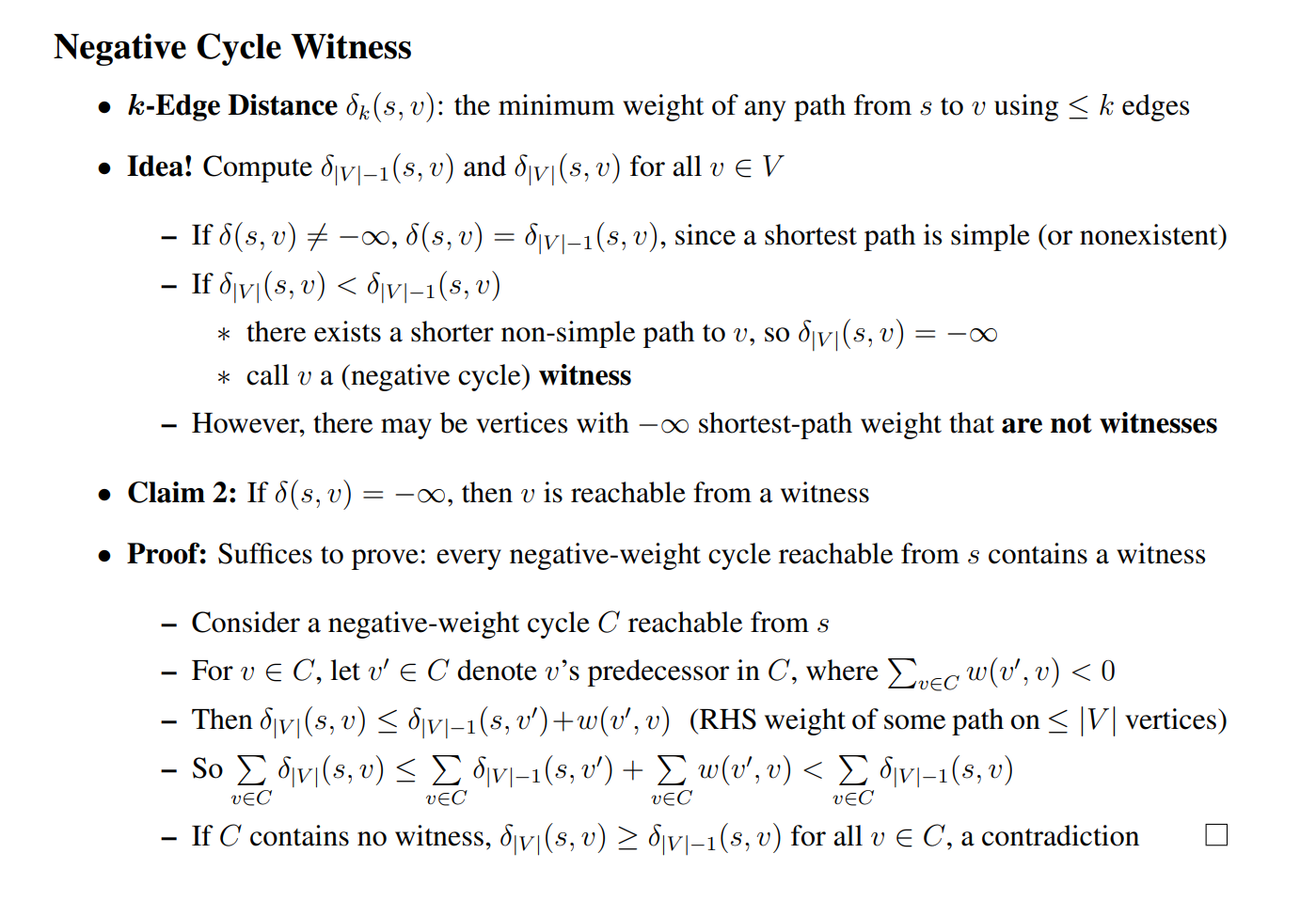

Claims

witness can be described as a vertex in the negative loop cycle.

Use graph duplication: make multiple copies (or levels) of the graph.

$|V| + 1$ levels: vertex $v_k $ in level $ k$ represents reaching vertex$ v$ from $s$ using $≤ k$ edges.

If edges only increase in levels, we can use DAG!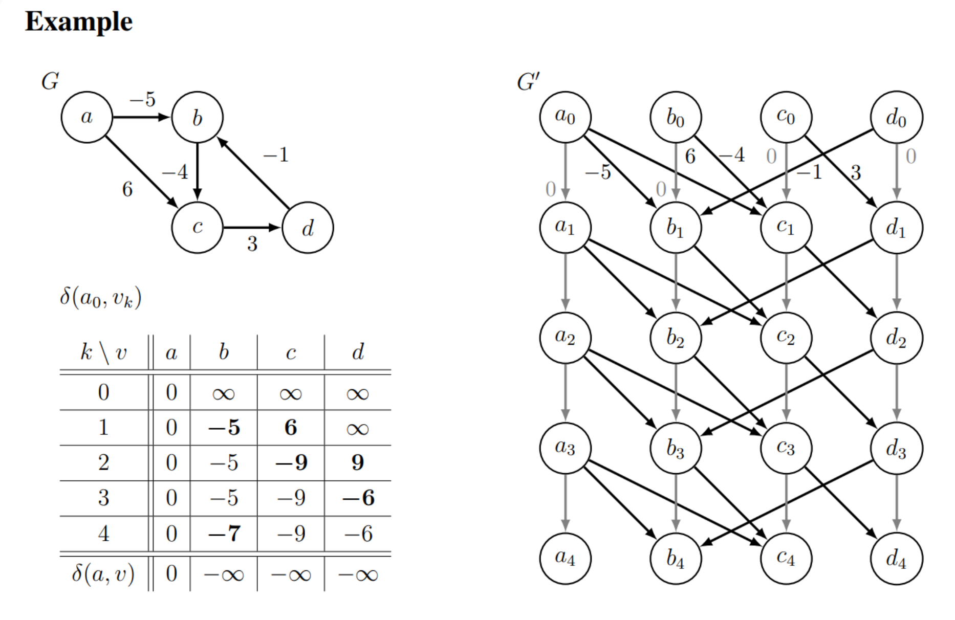

DAG

For the graph $G’$, it has $|V|\times |V + 1|$ vertices and $|V| \times |E|$ edges. And it is a directed graph! We can solve it using DAG with linear time. $O((|V| \times |E|)\times |V|)$.

Then we can use $\delta_{|V|}(s,v) < \delta_{|V|-1}(s,v)$ to judge whether it is $-\infty$.

$$\delta_k(s,v) = \delta’(s,v_k)$$.

Fix: Bellman-Ford Version 2

Dijkstra Algorithm

DAG:
- Best performance, linear time: $O(|V| + |E|)$.
- Restriction: cannot handle with circle path.
Bellman-Ford:
- $O(|V|(|V| + |E|))$
- for all kinds of graphs, general.
Dijkstra Algorithms: for non-negative weights, almost linear.

Intuition

Finally, I know it is SPFA…

We use Greedy Algorithms to handle the single shortest path problem. It makes locally optimal choices at each step with the intent of finding a globally optimal solution.

Like the DAG algorithms, we will start from the $w$, and maintain a Priority Queue to implement the greedy algorithms.

We will also use the triangle inequality, which is of the core principle for the greedy algorithms:

$$\text{dist}[v] \le \text{dist}[u] + w(u,v)$$

where $\text{dist}[u]$ means the shortest length from $w$ to $u$.

If we can ensure the correct path of $u$ will be calculated before the $v$, then we can ensure the rightness of $\text{dist}[v]$!

Pseudo Code

Loops

How greedy?: If $\text{dist}[v] \ge \text{dist}[u] + w(u,v)$, then upgrade the $\text{dist}[v]$ for the shorter path! It means that we don’t need to get the correct path for its first time! We can upgrade this during the upcoming process, and for the existence of the shortest path, we can unsure all the paths can be updated correctedly!

Time complexity

enqueue and dequeue: $O(|V| + |E|)$
For the enqueue and dequeue: $O(\log|V|)$

Hence the total time complexity: $O((|V| + |E|)\log(|V|))$

If we use Fibonacci heap: $O(|E| + |V|\log|V|)$

Restrictions

Why no-negative?

Because we need to ensure the greedy search is correct!

实际上，上文的Dijkstra算法是可以处理负权边的，因为其一个节点可以访问多次，代表着其值可以被不断的更新。并且我们会保证有穷最短路径的走法一定会被走到，因此我们可以保证最后答案的正确性。

但是在原始的Dijkstra算法中，会记录每一个节点是否被访问，并且不使用优先级队列来实现。（这个不同算法的实现方式不一样），如果记录每一个节点是否被访问，这个时候为了保证贪心算法的正确性，我们不可以处理负权边。

当然，肯定不可以处理 negative weight cycles.

Floyd Algorithms

在上文中的若干算法都是为了求解单源最短路问题，即Single source shortest path algorithms. 几种算法的时间复杂度如下：

传统的Dijkstra：$O(|E| + |V|\log|V|)$
Bellman-Ford: $O(|E||V|)$
- SPFA: $O(k|V|)$ (在大多数情况下，$k << |E|$)
DAG: $O(|E| + |V|)$

如果把问题推广，对于单词查询我希望任意给出两个节点$u$, $v$求其最短路，这如何实现？

如果使用上面的算法，复杂度如下：

Dijkstra * $|V|$ times: $O(|V|^2\log|V| + |E|)$
Bellman Ford: $O(|V|^2|E|)$

下面介绍Floyd算法，基于动态规划策略，时间复杂度为$O(|V|^3)$，这在稀疏图中可以达到很高的效率。

我们定义一个数组 f[k][x][y]，表示只允许经过结点$1$到$k$，结点$x$到结点$y$的最短路长度。

很显然，f[n][x][y] 就是结点$x$到结点$y$的最短路长度。我们的目标就是在递增$n$的同时记录信息。

状态转移方程

$$f[k][x][y] = min(f[k-1][x][y], f[k-1][x][k]+f[k-1][k][y])$$

从$k-1$的节点到允许使用$k$号节点，考虑：

$k$号节点被用做最短路的路径，即此时的最短路是$x \to \text{kth node} \to y$，根据最短路的性质，$x \to \text{kth node}$的最短路肯定和$x \to y$的最短路是重合的（因为能保证第k个节点一定在x到y的最短路中）
- 因此这一项就是: $f[k-1][x][k]+f[k-1][k][y]$
$k$号节点没有被用作最短路的路径，就是$f[k-1][x][y]$.

这就是Floyd算法的核心！

不过缺点显而易见：时空复杂度都非常高，因为我们需要维护非常庞大的状态数组。我们下面证明数组的第一位没有影响，即：

$$f[x][y] = min(f[x][y], f[x][k]+f[k][y])$$

对于给定的 k，当更新 f[k][x][y] 时，涉及的元素总是来自 f[k-1] 数组的第 k 行和第 k 列。然后我们可以发现，对于给定的 k，当更新 f[k][k][y] 或 f[k][x][k]，总是不会发生数值更新，因为按照公式 f[k][k][y] = min(f[k-1][k][y], f[k-1][k][k]+f[k-1][k][y]),f[k-1][k][k] 为 0，因此这个值总是 f[k-1][k][y]，对于 f[k][x][k] 的证明类似。

因此，如果省略第一维，在给定的 k 下，每个元素的更新中使用到的元素都没有在这次迭代中更新，因此第一维的省略并不会影响结果。

不过三层循环不可以省略，只是对空间的小优化：

for (k = 1; k <= n; k++) {
  for (x = 1; x <= n; x++) {
    for (y = 1; y <= n; y++) {
      f[x][y] = min(f[x][y], f[x][k] + f[k][y]);
    }
  }
}

拆点

分层图最短路，如：有$k$次零代价通过一条路径，求总的最小花费。

同样的，使用状态转移方程，$dis[i][j] = \min(\min(dis[\text{from}][j-1]), \min(dis[\text{from}][j] + w))$

其中$from$是$i$的父亲节点。

事实上，这个 DP 就相当于把每个结点拆分成了$k+ 1$个结点，每个新结点代表使用不同多次免费通行后到达的原图结点。换句话说，就是每个结点$u_i$表示使用 $i$ 次免费通行权限后到达 $u$ 结点。

Algorithm > SJTU CS0501(H) Data Structure

#tutorial #Finished #Data Structure #C/C++ #Graph

DataStructure Graph SSSP Problem

https://xiyuanyang-code.github.io/posts/DataStructure-Graph-SSSP-problem/

Author

Xiyuan Yang

Posted on

May 12, 2025

Updated on

May 19, 2025

Licensed under

Secure Shell and Encryption Previous

DataStructure Graph MST Problem Next