AINN Attention

Attention Mechanism

Introduction

由于笔者发现在讲解Transformer的网络架构的时候缺乏对前置知识的细致理解。走马观花式的学习终究还是假学习。

• 为什么RNN的Encoder-Decoder架构的表现不好？
• 为什么Transformer需要设计成矩阵？
• Q, K, V究竟代表什么意思？

因此，笔者下决心重起炉灶重构博客，尝试啃下这一块硬骨头。

今天的博客将会聚焦于Attention Mechanism的思想和数学实现。

Table of Contents

• 注意力机制
• RNN和seq2seq
• seq2seq和RNN的结合

Attention Mechanism

注意力机制是从生物学上获得的启发。应用到视觉世界中，威廉·詹姆斯提出了双组件框架，即人通过自主性提示和非自主性提示来选择性地引导注意力的焦点。

非自主性提示和自主性提示

• 非自主性提示：“显眼”的物品，视觉上最敏锐的部分，获得直接的感官感受。
• 自主性提示：受到认知和意识的控制。

例如，

• 我因为Macbook图标很亮眼而注意到它：非自主性提示。（直接的感官感受）
• 我因为想到要去买苹果而注意到桌上的苹果。（自主性提示，收到自我意识的驱动）

查询，键和值

如果建模这两种注意力机制？这是神经科学家非常关心的问题。

显然，对于非自主性提示，本质就是图片的特征提取，我们可以使用卷积核和卷积神经网络来提取图片中的特征（例如高亮度区域，色彩鲜艳的区域，锐度高的区域等等），不是我们今天讨论的重点。

但是对于自主性提示，其机制相对更加复杂。并且在现实世界中注意力往往是两种提示相互夹杂的。我们可以使用如下的基本结构来进行建模：

对于人类一般性的行为，我们可以建模成：

$$\boxed{\text{attention}} \to \boxed{\text{sensory input}} \to \boxed{\text{output}}$$

视觉上产生了注意力（自主 & 非自主），接着在大脑皮层产生感觉，并做出对应的输出。

• 翻译：接受视觉输入 $\to$ 在脑海中产生感觉（思考的过程） $\to$ 输出成另一种语言

当我们看到一幅画中的苹果，可能会联想到吃苹果的甜味，甚至不自觉流口水。这一过程可以用注意力机制来解释，涉及三个核心概念：

1. 查询（Query）：当前的感知输入，如画中苹果的视觉特征（颜色、形状等），它触发大脑的检索机制（就是非自主性提示）。
2. 键（Key）：长期记忆中的关联信息，如过去吃苹果的经验。大脑会计算Query和Key的匹配程度，选择最相关的记忆。
3. 值（Value）：被选中的Key对应的具体信息，如“苹果是甜的”，进而触发味觉联想和生理反应。

这一机制的关键在于：

• 选择性：并非所有记忆都会被激活，只有与当前输入最相关的信息才会被提取。
• 联想性：视觉输入（Query）通过匹配记忆（Key）触发跨模态体验（Value），如“看到苹果→想到甜味”。
• 自动化：该过程通常是快速、无意识的，体现大脑的高效信息检索能力。

通过这种机制，外部刺激（如画面）能自动激活相关记忆，并影响认知和生理反应。

在注意力机制中，自主性提示被称为查询（query），而非自主性提示（客观存在的咖啡杯和书本）作为键（key）与感官输入（sensory inputs）的值（value）构成一组 pair 作为输入。而给定任何查询，注意力机制通过注意力汇聚（attention pooling）将非自主性提示的 key 引导至感官输入。

• 例如在RNN中，隐藏状态H是自主性提示，而新的input就是非自主性提示。
  • 如果不更新隐藏状态，而是直接对序列进行暴力建模，就相当于只考虑到非自主性提示，就是经典的MLP！

来点抽象的！我们给定键值对$(x_i, y_i)$，并给出需要查询的$x_q$(query)，我们需要输出$\hat{y}=f(x_q)$作为我们的输出值。

$f$就是注意力机制的黑箱函数，给定好框架之后的创新无非就是针对对于$f$的函数的设计。

注意力汇聚算法

我们不妨设计一些简单的$f$，来看看效果怎么样。最简单的设计就是平均估计个体，即使用Average Pooling的操作：

$$f(x_q) = \frac{1}{n} \sum_{i= 1}^{n}y_i$$

这细细一想就很扯淡，因为这样无论给出什么样的query输出的结果总是一样的，bullshit！

也就是说，我们希望在输出预测的时候尽可能的使用到已知的信息，即我们所知道的键值对$(x_i, y_i)$。一个很自然的想法是**判断$x_q$和每一个键$x_i$**的相关程度，并以此为基础作为权重，再加权平均所有的$y_i$。

例如我从Query为“画中的苹果”检索到脑海中的苹果，可以认为是这两个事物的相关性很强，因此权重非常大，最后的输出就几乎全是“脑海中的苹果”对应的值。如果我的query是“画中那个洒满椒盐的苹果”，那可能这和脑海中“椒盐”这个键的相关性就会大幅度上升，进而产生相对应（值）的咸咸的感觉。

我们便得到了注意力汇聚公式（Attention Pooling），本质上就是加一个与键有关的权重，没什么特别的：

$$f(x_q) = \sum_{i= 1}^{n} \alpha(x_q, x_i) y_i,\ \sum_{i = 1}^{n}\alpha(x_q, x_i) = 1 $$

如何设计权重？考虑相关性，因此我们可以对$\alpha(x_q, x_i)$进一步细化，我们假设$K(x_i,x_j)$衡量了两个向量的相关性：

$$\alpha(x_q, x_i) = \frac{K(x_q, x_i)}{\sum_{j = 1}^{n}K(x_q, x_j)}$$

更进一步，如果我们考虑高斯核公式（先考虑一阶的）：

$$\alpha(x_q,x_i) = \frac{\exp(-\frac{1}{2}(x_q - x_i)^2)}{\sum_{j = 1}^{n}\exp(-\frac{1}{2}(x_q - x_j)^2)} = \text{softmax}(-\frac{1}{2}(x_q - x_i)^2)$$

那我们就可以得到一个具体化的$f(x)$：

$$\hat{y} = f(x) = \sum_{i = 1}^{n} \text{softmax}(-\frac{1}{2}(x_q - x_i)^2) y_i$$

更进一步，我们希望这个函数可以携带可被学习的参数：

$$\hat{y} = f(x) = \sum_{i = 1}^{n} \text{softmax}(-\frac{1}{2}((x_q - x_i)\omega)^2) y_i$$

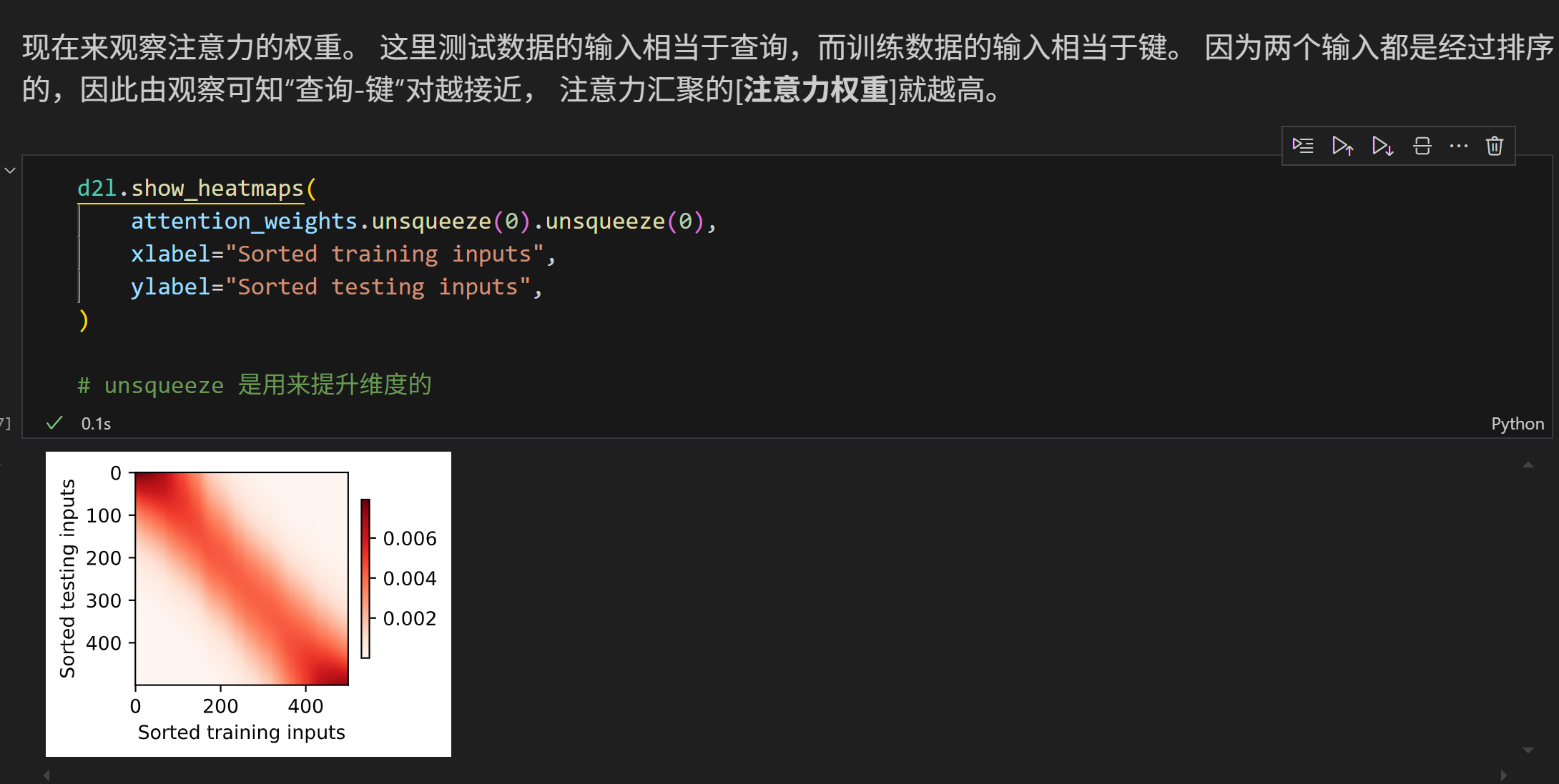
热力图显示当key和query越接近的时候，其权重更高。（这里是一维的情况，就直接比较两个值的大小）

但是带权重的注意力汇聚在做梯度下降的时候会出现不平滑的现象（虽然loss确实下降了），因为在键值对很小的情况下很容易出现过拟合的情况。

可以理解为在一些有噪声的点附近，由于过拟合的存在（额外参数的影响）让这个点的权重变大了，导致heatmap出现了断点处的偏移。

这里引用一个非常好的回答：参数化的意义是什么

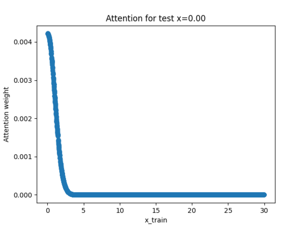
增加权重的意义在于使得对于远距离的key有着更小的关注，缩小的注意力的范围。

Adding Batches

为了充分发挥GPU的并行优势，我们可以使用批量矩阵的乘法。

假设现在有$n$个$(a,b)$的二维矩阵$X_i(1\le i \le n)$和$n$个$(b,c)$的二维矩阵$Y_i(1\le i \le n)$，在非并行的状态下，我们需要做$n$次顺序矩阵乘法，即$X_i \times Y_i:=A_i$，最终得到$n$个$(a,c)$的矩阵。

并行的本质就是大家一起做运算，把$n$个$(a,b)$的二维矩阵$X_i(1\le i \le n)$可以定义为三维张量$T$，size是$(n,a,b)$。

因此，**假定两个张量的形状分别是$(n,a,b)$和$(n,b,c)$，它们的批量矩阵乘法输出的形状为$(n,a,c)$**。

如何使用小批量乘法来改写注意力机制？

计算加权平均值的过程可以看做是两个向量的内积操作（需要归一化），因此假设每一次批量是size为$n$，那么：

$$\text{Weight(n, 1, len)} \times \text{Value(n, len, 1)} = \text{Score(n,1)}$$

$n$在实际情况下可以定义为查询的个数，$len$是键值对的个数。

很惊讶的发现在这里$len$和$n$是无关的量，即我们可以不断的scale up键值对的个数，即获得更多的采样。

批量矩阵乘法在这里可以计算小批量数据的加权平均值。

# orginal weights and values
weights = torch.ones((2,10)) * 0.1
values = torch.arange(20.0).reshape((2,10))
# weight: torch.Size([2, 10])
# values: torch.Size([2, 10])

# compute in sequential order
all_answer = torch.Tensor()
for i in range(0,weights.shape[0]):
    weights_single = weights[i]
    values_single = values[i]
    answer = weights_single.dot(values_single.T).unsqueeze(-1)
    all_answer = torch.cat([all_answer, answer])

# custom the size
all_answer1 = all_answer.unsqueeze(-1).unsqueeze(-1)

# using torch.bmm
weights = weights.unsqueeze(1)
# weights: [2,1,10]
values = values.unsqueeze(-1)
# values: [2,10,1]
all_answer2 = torch.bmm(weights, values)

assert torch.allclose(all_answer1, all_answer2)

Code: Nadaraya-Waston Kernel

在这个部分，我们将要实现最基本的注意力汇聚算法来尝试拟合一个函数，数学原理如上文所呈现：

不带参数的版本：

$$\hat{y} = f(x) = \sum_{i = 1}^{n} \text{softmax}(-\frac{1}{2}(x_q - x_i)^2) y_i$$

带参数的版本：

$$\hat{y} = f(x) = \sum_{i = 1}^{n} \text{softmax}(-\frac{1}{2}((x_q - x_i)\omega_i)^2) y_i$$

注意，这里和书上的公式有点不太一样，书上只引入了一个标量参数$w$，导致非常容易出现过拟合的现象，这里的可学习参数$\vec{\mathbf{w}} = \{w_1, w_2, w_3,\dots,w_n\}$，其中$n$是预先定义好的键值对的个数。

代码如下，主要的核心逻辑是：

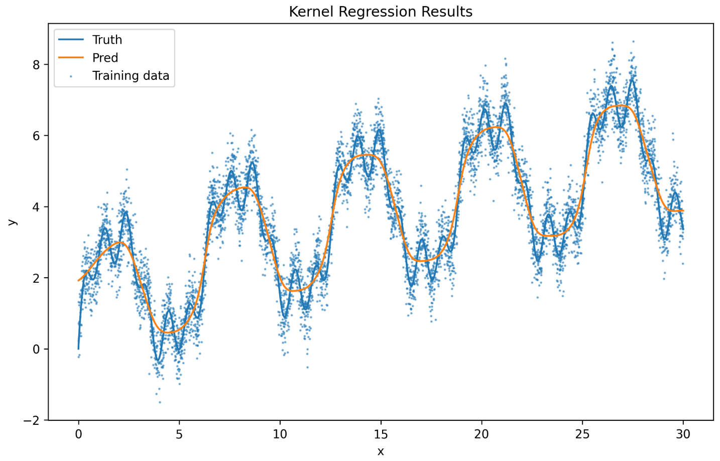
• 生成数据集，我们需要拟合的函数是$f(x) = 2\sin(x) + 0.4\sin(3x) + 0.6\sin(6x) + \sqrt{x}$
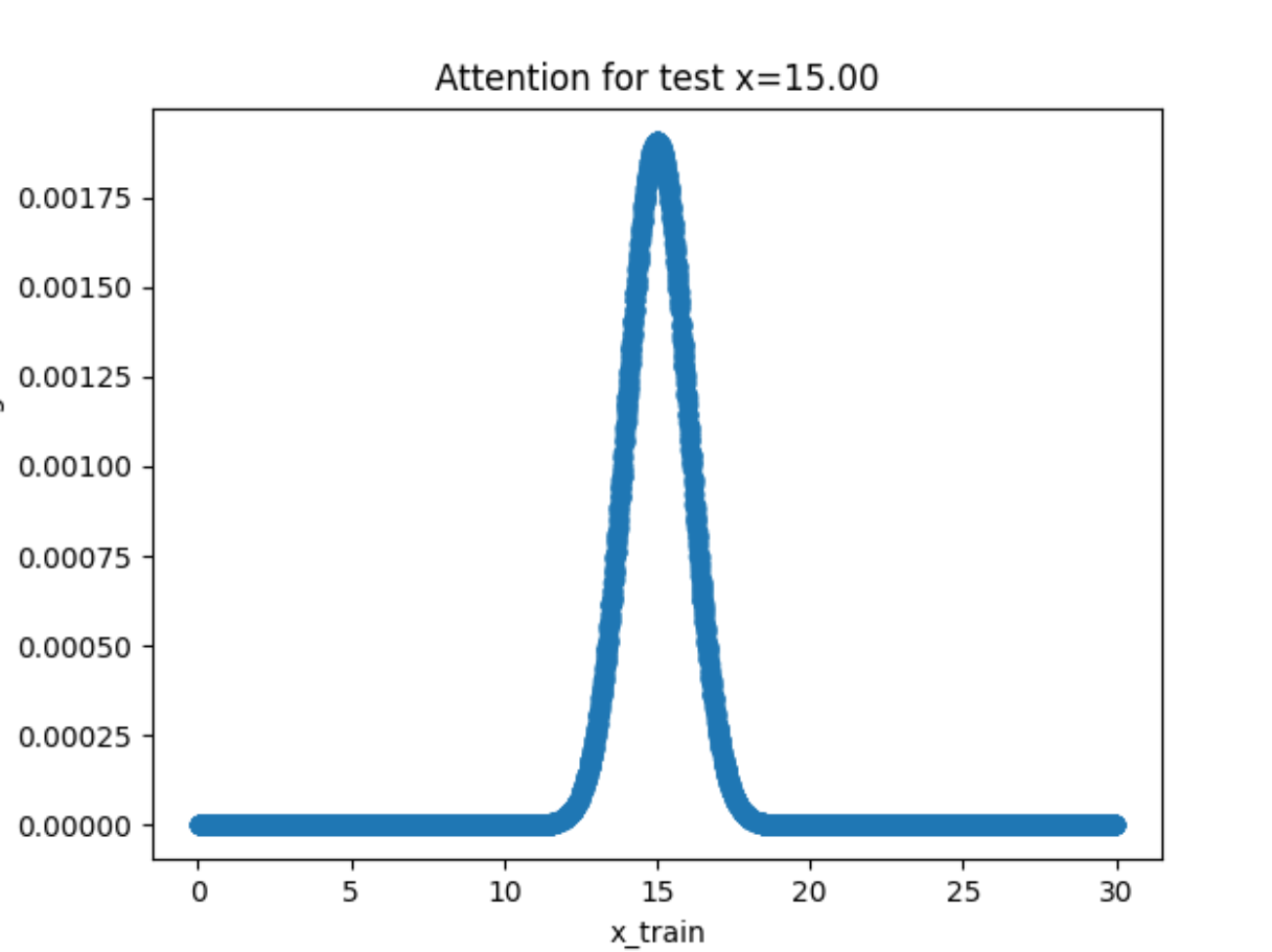
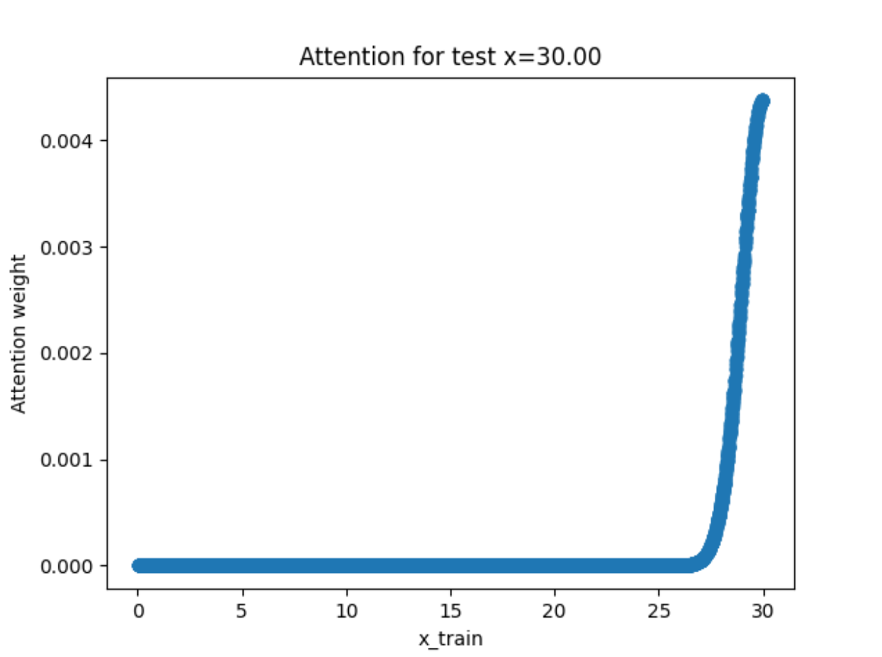
• 首先直接根据不带参数的版本，即没有任何的可训练参数，直接生成test的结果。
• 接下来使用带参数的版本进行梯度下降训练，得到第二个拟合结果。

import torch.nn as nn
import torch
import torch.nn.functional as F
import matplotlib.pyplot as plt
import os
import numpy as np

os.environ["CUDA_VISIBLE_DEVICES"] = "0,1,2,3"


def show_heatmaps(
    matrices,
    xlabel="Keys",
    ylabel="Queries",
    titles=None,
    figsize=(6, 6),
    cmap="Reds",
    save_path=None,
):
    """
    Display heatmaps for attention weights or other matrices.

    Args:
        matrices: Input tensor or array of shape (num_rows, num_cols, height, width)
        xlabel: Label for x-axis
        ylabel: Label for y-axis
        titles: List of titles for subplots
        figsize: Size of the figure
        cmap: Color map
        save_path: Path to save the figure (None for not saving)
        show: Whether to display the figure
    """
    # Convert PyTorch tensor to numpy array if needed
    if hasattr(matrices, "detach"):
        matrices = matrices.detach().cpu().numpy()

    num_rows, num_cols = matrices.shape[0], matrices.shape[1]

    # Create figure and axes
    fig, axes = plt.subplots(
        num_rows, num_cols, figsize=figsize, sharex=True, sharey=True, squeeze=False
    )

    # Plot each matrix
    for i in range(num_rows):
        for j in range(num_cols):
            pcm = axes[i, j].imshow(matrices[i, j], cmap=cmap)

            # Add labels only to the bottom row and leftmost column
            if i == num_rows - 1:
                axes[i, j].set_xlabel(xlabel)
            if j == 0:
                axes[i, j].set_ylabel(ylabel)

            # Add titles if provided
            if titles is not None:
                axes[i, j].set_title(titles[j])

    fig.savefig(save_path, dpi=300, bbox_inches="tight")

    # Close the figure to prevent memory leaks
    plt.close()


def plot_kernel_reg(
    y_hat, x_test, y_truth, x_train, y_train, save_path="img/kernel_regression.png"
):
    """
    Plot kernel regression results and save the figure.

    Args:
        y_hat: Predicted values (tensor or array)
        x_test: Test input values
        y_truth: Ground truth values for test inputs
        x_train: Training input values
        y_train: Training target values
        save_path: Path to save the figure (default: "img/kernel_regression.png")
    """
    # Convert tensors to numpy if needed
    if hasattr(y_hat, "detach"):
        y_hat = y_hat.detach().cpu().numpy()
    if hasattr(y_truth, "detach"):
        y_truth = y_truth.detach().cpu().numpy()
    if hasattr(x_test, "detach"):
        x_test = x_test.detach().cpu().numpy()
    if hasattr(x_train, "detach"):
        x_train = x_train.detach().cpu().numpy()
    if hasattr(y_train, "detach"):
        y_train = y_train.detach().cpu().numpy()

    # Create figure
    plt.figure(figsize=(10, 6))

    # Plot truth and prediction lines
    plt.plot(x_test, y_truth, label="Truth")
    plt.plot(x_test, y_hat, label="Pred")

    # Plot training data points
    plt.scatter(x_train, y_train, marker="o", alpha=0.5, s=1, label="Training data")

    # Add labels and legend
    plt.xlabel("x")
    plt.ylabel("y")
    plt.title("Kernel Regression Results")
    plt.legend()

    # Save figure with high quality
    plt.savefig(save_path, dpi=300, bbox_inches="tight")
    plt.close()


def generate_datasets(width: float, n_train: int, n_test: int):
    """Generate random datasets for NWKernel regression."""
    x_train = torch.sort(torch.rand(n_train) * width).values

    def target_function(x):
        return (
            2 * torch.sin(x) + 0.4 * torch.sin(3 * x) + 0.6 * torch.sin(6 * x) + x**0.5
        )

    y_train = target_function(x_train) + torch.normal(0.0, 0.5, (n_train,))
    x_test = torch.linspace(0, width, n_test)
    y_truth = target_function(x_test)

    print(f"Generated datasets - Train: {n_train}, Test: {n_test}")
    return x_train, y_train, x_test, y_truth


class NWKernelRegression(nn.Module):
    def __init__(self, x_train, y_train):
        super().__init__()
        self.register_buffer("x_train", x_train)
        self.register_buffer("y_train", y_train)
        # We use one weight per training example
        self.w = nn.Parameter(torch.ones(len(x_train)), requires_grad=True)

    def forward(self, queries):
        queries = queries.unsqueeze(1)  # [n_queries, 1]
        keys = self.x_train.unsqueeze(0)  # [1, n_train]
        diff = queries - keys  # [n_queries, n_train]
        self.attention_weights = F.softmax(-((diff * self.w) ** 2) / 2, dim=1)
        return torch.matmul(self.attention_weights, self.y_train)


def visualize_attention(
    net, x_test, x_train, num_points=3, save_path="img/visualize_attention.png"
):
    """Visualize attention weights for a few test points."""

    idxs = torch.linspace(0, len(x_test) - 1, num_points).long()
    queries = x_test[idxs]
    keys = x_train
    w_cpu = net.w.detach().cpu()
    keys_cpu = keys.detach().cpu() if hasattr(keys, "detach") else torch.tensor(keys)
    with torch.no_grad():
        for i, query in enumerate(queries):
            query_cpu = (
                query.detach().cpu()
                if hasattr(query, "detach")
                else torch.tensor(query)
            )
            diff = query_cpu - keys_cpu
            attn = torch.softmax(-(diff * w_cpu).pow(2) / 2, dim=0)
            plt.figure()
            plt.title(f"Attention for test x={query_cpu.item():.2f}")
            plt.plot(keys_cpu, attn.numpy(), "o-")
            plt.xlabel("x_train")
            plt.ylabel("Attention weight")
            plt.savefig(save_path)
            plt.close()


def visualize_kernel_shape(net, x_train, save_path="img/kernelshape_visualize.png"):
    """Visualize the learned kernel shape centered at a point."""
    import matplotlib.pyplot as plt

    center = x_train[len(x_train) // 2]
    diffs = torch.linspace(-5, 5, 100)
    w_mean_cpu = net.w.mean().detach().cpu()
    with torch.no_grad():
        attn = torch.softmax(-(diffs * w_mean_cpu).pow(2) / 2, dim=0)
    plt.figure()
    plt.title("Learned Kernel Shape")
    plt.plot(diffs.numpy(), attn.numpy())
    plt.xlabel("x - center")
    plt.ylabel("Kernel value")
    plt.savefig(save_path)
    plt.close()


def visualize_training_process(
    record_epoch, record_loss, save_path="img/visualize_training_process.png"
):
    plt.figure()
    plt.title("Training Process")
    plt.plot(record_epoch, record_loss)
    plt.xlabel("epoches")
    plt.ylabel("Training Loss")
    plt.savefig(save_path)
    plt.close()


def train(width, epochs, n_train, n_test, x_train, y_train, x_test, y_truth):
    # Move data to GPU if available
    device = torch.device("cuda" if torch.cuda.is_available() else "cpu")
    x_train = x_train.to(device)
    y_train = y_train.to(device)
    x_test = x_test.to(device)
    y_truth = y_truth.to(device)

    # Initialize model and optimizer
    net = NWKernelRegression(x_train, y_train).to(device)

    if torch.cuda.device_count() > 1:
        print(f"Using {torch.cuda.device_count()} GPUs for DataParallel.")
        net = nn.DataParallel(net)

    criterion = nn.MSELoss()
    optimizer = torch.optim.SGD(net.parameters(), lr=0.5)
    record_loss = []
    record_epochs = []

    plot_epochs = {
        10,
        100,
        1000,
        5000,
        10000,
        20000,
        50000,
        60000,
        70000,
        80000,
        100000,
        110000,
        120000,
    }

    for epoch in range(epochs):
        optimizer.zero_grad()
        y_pred = net(x_train)
        loss = criterion(y_pred, y_train)
        loss.backward()
        optimizer.step()

        record_loss.append(loss.item())
        record_epochs.append(epoch)

        if epoch % 10 == 0:
            print(f"Epoch {epoch}, Loss: {loss.item():.4f}")

        if (epoch + 1) in plot_epochs:
            with torch.no_grad():
                y_hat = (
                    net.module(x_test)
                    if isinstance(net, nn.DataParallel)
                    else net(x_test)
                )
            plot_kernel_reg(
                y_hat.cpu(),
                x_test.cpu(),
                y_truth.cpu(),
                x_train.cpu(),
                y_train.cpu(),
                save_path=f"img/kernel_regression_epoch{epoch+1}.png",
            )

    visualize_training_process(record_epochs, record_loss)

    # Testing
    with torch.no_grad():
        y_hat = net.module(x_test) if isinstance(net, nn.DataParallel) else net(x_test)

    model_for_vis = net.module if isinstance(net, nn.DataParallel) else net
    plot_kernel_reg(
        y_hat.cpu(), x_test.cpu(), y_truth.cpu(), x_train.cpu(), y_train.cpu()
    )
    visualize_attention(model_for_vis, x_test.cpu(), x_train.cpu())
    visualize_kernel_shape(model_for_vis, x_train.cpu())

    show_heatmaps(
        model_for_vis.attention_weights.unsqueeze(0).unsqueeze(0).cpu(),
        xlabel="training inputs",
        ylabel="testing inputs",
        titles="HeatMaps for the final attention",
        save_path="img/heatmap_params.png"
    )


def singleNWKernel(width, n_train, n_test, x_train, y_train, x_test, y_truth):
    sigma = 1.0  # fixed kernel size
    x_train_cpu = x_train.cpu()
    y_train_cpu = y_train.cpu()
    x_test_cpu = x_test.cpu()
    y_truth_cpu = y_truth.cpu()

    # compute attention weights
    queries = x_test_cpu.unsqueeze(1)  # [n_test, 1]
    keys = x_train_cpu.unsqueeze(0)  # [1, n_train]
    diff = queries - keys  # [n_test, n_train]
    attn = torch.softmax(-((diff / sigma) ** 2) / 2, dim=1)  # 固定sigma
    y_hat = torch.matmul(attn, y_train_cpu)

    plot_kernel_reg(
        y_hat,
        x_test_cpu,
        y_truth_cpu,
        x_train_cpu,
        y_train_cpu,
        save_path="img/kernel_regression_noparam.png",
    )

    def visualize_attention_noparam(
        x_test,
        x_train,
        attn,
        num_points=3,
        save_path="img/visualize_attention_noparam.png",
    ):
        idxs = torch.linspace(0, len(x_test) - 1, num_points).long()
        for i, idx in enumerate(idxs):
            plt.figure()
            plt.title(f"Attention for test x={x_test[idx].item():.2f}")
            plt.plot(x_train, attn[idx].numpy(), "o-")
            plt.xlabel("x_train")
            plt.ylabel("Attention weight")
            plt.savefig(f"img/visualize_attention_noparam_{i}.png")
            plt.close()

    visualize_attention_noparam(x_test_cpu, x_train_cpu, attn)

    def visualize_kernel_shape_noparam(
        sigma, save_path="img/kernelshape_visualize_noparam.png"
    ):
        diffs = torch.linspace(-5, 5, 100)
        attn = torch.softmax(-(diffs / sigma).pow(2) / 2, dim=0)
        plt.figure()
        plt.title("Fixed Kernel Shape")
        plt.plot(diffs.numpy(), attn.numpy())
        plt.xlabel("x - center")
        plt.ylabel("Kernel value")
        plt.savefig(save_path)
        plt.close()

    visualize_kernel_shape_noparam(sigma)

    show_heatmaps(
        attn.unsqueeze(0).unsqueeze(0),
        xlabel="training inputs",
        ylabel="testing inputs",
        titles="HeatMaps for the final attention (no param)",
        save_path="img/heatmap_noparam.png",
    )


if __name__ == "__main__":
    # Parameters
    width = 20.0
    n_train = 6000
    n_test = 6000
    epochs = 120001

    # Run tests
    x_train, y_train, x_test, y_truth = generate_datasets(width, n_train, n_test)
    # Train and evaluate
    print("For models with no parameters")
    singleNWKernel(
        width=width,
        n_train=n_train,
        n_test=n_test,
        x_train=x_train,
        y_train=y_train,
        x_test=x_test,
        y_truth=y_truth
    )

    print("For models with parameters")
    train(width, epochs, n_train, n_test, x_train, y_train, x_test, y_truth)

实验结果分析

首先来看不带参数的版本：

因为没有参数，所以图像都非常的平滑！（这其实也是因为数据点采样的均匀性）但是从回归图像可以看出拟合的效果并不好，尤其在有噪声的情况下。

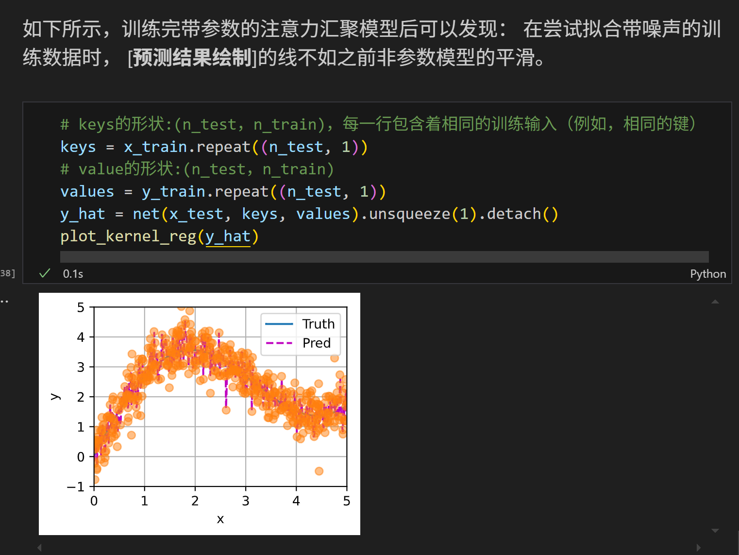
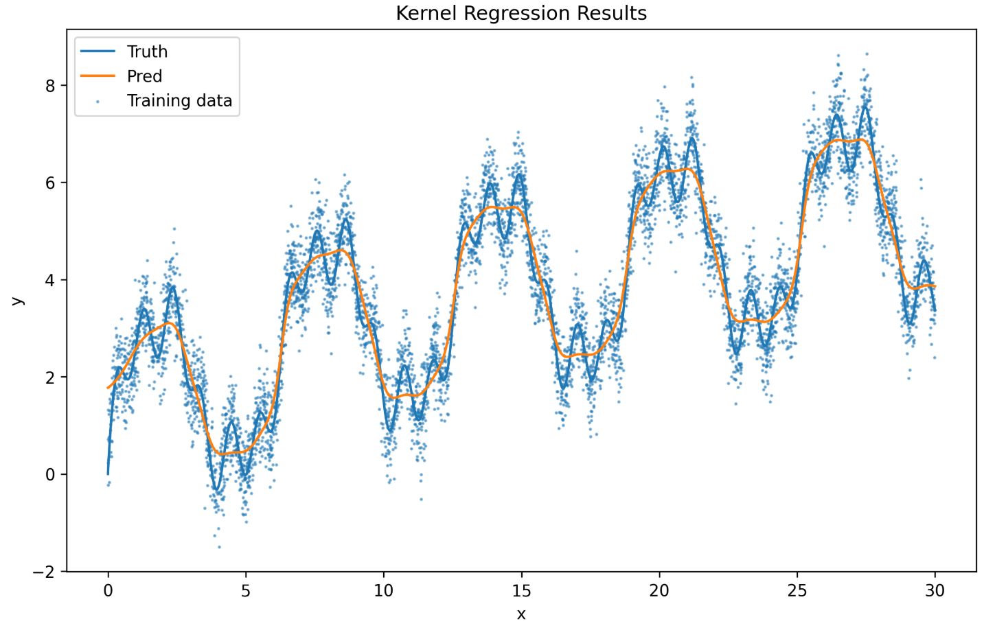
再来看带参数的版本：

下面三张图片分别是训练5000,50000,120000个epoch之后的版本。

其实这里也还是存在过拟合的问题，函数的参数过小，在后面的epoch发生了梯度消失的现象。

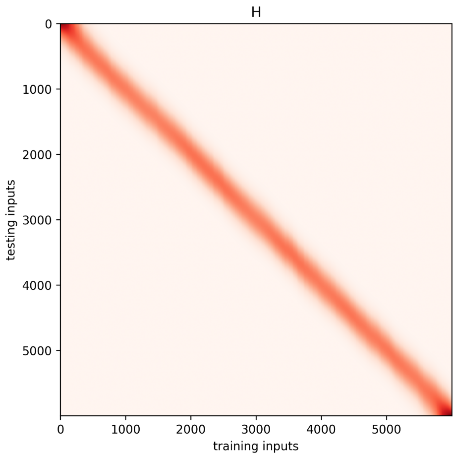
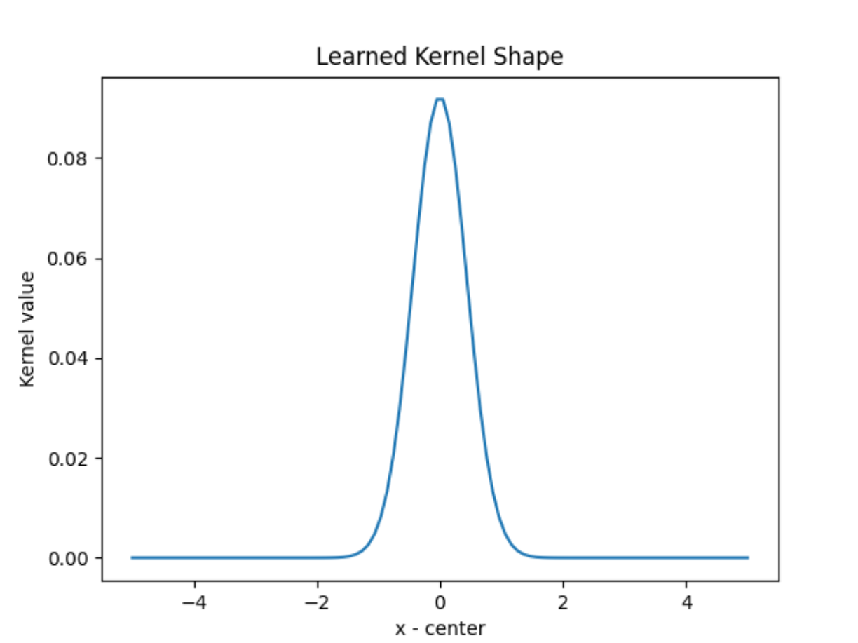
从Kernel Shape也可以看出，参数的引入是的距离效应显得更显著，即距离近的点的权重更大，而距离远的点的权重变得更小。

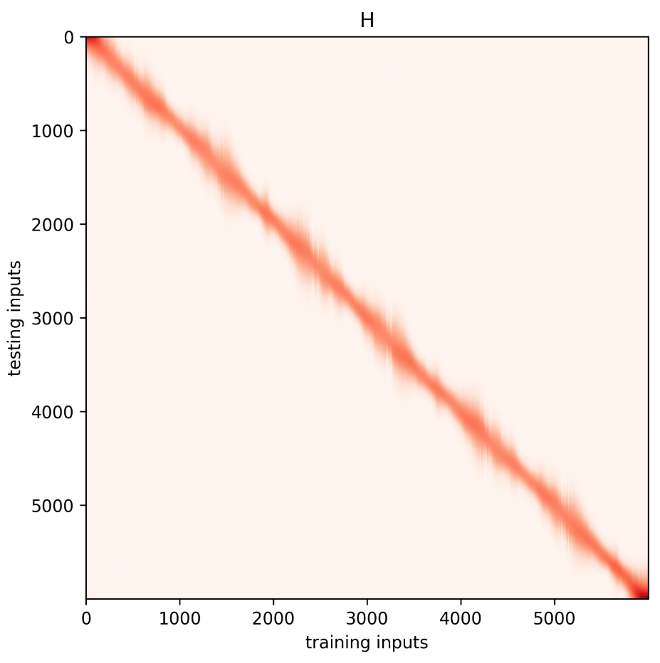
如果看热力图可以发现，参数的引进导致图像变的模糊，这也是数据采样点的效果。

注意力评分函数

上文的公式：

$$\alpha(x_q,x_i) = \frac{\exp(-\frac{1}{2}(x_q - x_i)^2)}{\sum_{j = 1}^{n}\exp(-\frac{1}{2}(x_q - x_j)^2)} = \text{softmax}(-\frac{1}{2}(x_q - x_i)^2)$$

可以作为一个注意力评分函数，用来衡量查询值$x_q$和单个键值$x_i$的相关性。

我们可以推广到更加高维的空间中：

考虑查询$\vec{\mathbf{q}} \in \mathbb{R}^q$（在$q$维空间中），我们有$m$个键值对：$(\vec{\mathbf{k_1}}, \vec{\mathbf{v_1}})$, $(\vec{\mathbf{k_2}}, \vec{\mathbf{v_2}})$, … , $(\vec{\mathbf{k_m}}, \vec{\mathbf{v_m}})$, 其中$\vec{\mathbf{k_i}} \in \mathbb{R}^k$, $\vec{\mathbf{v_i}} \in \mathbb{R}^v$。

注意这里的键和值都被推广位高维空间下的向量，并且向量可以是不同维度的（可以粗糙的理解：翻译前后文本语义空间并不相同）

那么我们可以做如下的推广计算每一个查询的权重。

$$f(\mathbf{q}, (\mathbf{k_1}, \mathbf{v_1}), \ldots, (\mathbf{k_m}, \mathbf{v_m})) = \sum_{i=1}^m w_i \mathbf{v}_i \in \mathbb{R}^v$$

$$f(\mathbf{q}, (\mathbf{k_1}, \mathbf{v_1}), \ldots, (\mathbf{k_m}, \mathbf{v_m})) = \sum_{i=1}^m \alpha(\mathbf{q}, \mathbf{k_i}) \mathbf{v_i} \in \mathbb{R}^v$$

$$\alpha(\mathbf{q}, \mathbf{k_i}) = \mathrm{softmax}(a(\mathbf{q}, \mathbf{k_i})) = \frac{\exp(a(\mathbf{q}, \mathbf{k_i}))}{\sum_{j=1}^m \exp(a(\mathbf{q}, \mathbf{k_j}))} \in \mathbb{R}$$

注意这里的$w_i$是一个标量，也是$\alpha(\mathbf{q}, \mathbf{k}_i)$的输出。

显然，在更加general的任务上，$q,k,v$的三个维度指标往往不相同。这就导致了维度不匹配的情况，单纯的NWKernel公式需要在维度对齐的情况下进行运算（比较两个向量的余弦相似度），因此后人工作的重点就是如何设计更好的 注意力评分函数 $\alpha(\mathbf{q}, \mathbf{k}_i)$。下文介绍两种经典的算法：加性注意力和缩放点积注意力，以及Bahdanau注意力。

注意力加性函数本身不需要考虑归一化的处理方式，因为后面会套一个softmax层。

掩蔽softmax操作

回到机器翻译的问题上，在使用注意力模型的时候，为了提高效率采用批量处理的形式（方便矩阵并行运算），但是可能会存在同一批次文本序列长度不一致的问题，这个时候常用的方法是短序列使用特殊字符填充，即做padding；此外在做序列生成时，我们不希望机器依赖未来的词元做“抄袭”。以上两种情况本质上即为不希望全部的key被纳入模型考虑的范围内（例如特殊字符padding的部分&未来词元等），换句话说，我们需要设置有效长度，超过有效长度的键值对采用掩蔽操作，忽略其对模型的影响。

掩蔽的过程在softmax层进行，注意力评分正常计算，但是在进入softmax归一化的时候，对每一个维度设置需要掩蔽的valid_length，因此需要传递进去一个张量，表示每一个批量的valid length，代码见教材，下面给出一个示例：

# test_tensor 的维度是(2,2,4)
print(masked_softmax(test_tensor, torch.tensor([2,3])))

这里第一个维度2是batchsize，第2个维度是query的数量，第三个维度是键的数量，这里有点容易搞混。

这里做softmax是对最后一个维度的行向量做的，因此在下面的结果也可以看到每一行的和为1

tensor([[[ 0.4140, -1.1542, -1.2127,  0.6286],
         [-0.6033,  0.5189, -1.4756, -0.0650]],

        [[-0.1864,  0.5557,  0.1935, -1.2823],
         [ 0.1995, -1.6036,  1.3123, -0.0660]]])
tensor([[[0.8275, 0.1725, 0.0000, 0.0000],
         [0.2456, 0.7544, 0.0000, 0.0000]],

        [[0.2192, 0.4604, 0.3205, 0.0000],
         [0.2377, 0.0392, 0.7232, 0.0000]]])

例如这里矩阵的第一个维度为2（批量数），对于第一个批量，掩蔽有效长度为2，那么对这个二维矩阵的第三列即之后的列元素都做掩蔽操作，对于第二个批量掩蔽的有效程度为3，显然第四列被做了掩码处理。

加性注意力

说到底，设计一个好的注意力函数关键在于设计函数：

$$a(\mathbf{q},\mathbf{k_i}) \in \mathbb{R}, \mathbf{q} \in \mathbb{R}^{q}, \mathbf{k_i} \in \mathbb{R}^{k}$$

即衡量两个不同维度空间下向量的相似度问题。

加性注意力的做法是同样扩展到相同维度$h$的向量空间,即：

$$a(\mathbf{q},\mathbf{k_i}) = \mathbf{\omega_{v}}^{\top} \tanh(W_q \mathbf{q}+W_k\mathbf{k} + \mathbf{b}) \in \mathbb{R}, W_q \in \mathbb{R}^{h \times q}, W_k \in \mathbb{R}^{h \times k}, \mathbf{\omega_{v}}^{\top} \in \mathbb{R}^h $$

其实就是一个多层感知机…包含一个参数为h的隐藏层，独特的点是存在两个维度迁移的可学习矩阵，进而实现维度的统一后“加性”拼接。

包含一个隐藏层的感知机的形式化表达：

$$ \hat{y} = \sigma( \mathbf{W_2} ( \sigma(\mathbf{W_1} \mathbf{x} + \mathbf{b_1}) ) + \mathbf{b_2})$$

在加性注意力中输入的向量就是$\mathbf{q}$和$\mathbf{k}$，从输入层到隐藏层的激活函数是$\tanh$，从隐藏层到输出层再做一个比较简单的点积处理。

同时，加性注意力一般会禁用偏置项。

class AdditiveAttention(nn.Module):
    """加性注意力"""
    def __init__(self, key_size, query_size, num_hiddens, dropout, **kwargs):
        # 相关参数的意义：
        # W_k代表k的可学习矩阵，将key_size映射到num_hiddens的维度
        # W_q代表q（查询）的可学习矩阵，将query_size维度映射到num_hiddens的维度
        # w_v代表最后输出层的参数，将num_hiddens维度映射到单个维度

        # *这里调用其他的参数**kwargs传递给父类nn.Module的构造函数
        super(AdditiveAttention, self).__init__(**kwargs)
        self.W_k = nn.Linear(key_size, num_hiddens, bias=False)
        self.W_q = nn.Linear(query_size, num_hiddens, bias=False)
        self.w_v = nn.Linear(num_hiddens, 1, bias=False)
        self.dropout = nn.Dropout(dropout)

    def forward(self, queries, keys, values, valid_lens):
        # 考虑批量处理，queries，keys和values都是3维张量
        # queries: (batch_size, query_num, query_size), 其中query_size是向量的维度
        # keys: (batch_size, 键值对的个数, key_size)
        # 为了方便后续的维度对齐，扩展到四个维度（后续代码unsqueeze的操作）
        # !其实这里是先做的映射在做的维度扩展
        # *queries: (batch_size, query_num, 1, query_size)
        # *key: (batch_size, 1, 键值对的个数, key_size)

        # ! 这一步对上述的两个四维张量的最后一个维度做映射操作，改变最后一个维度
        queries, keys = self.W_q(queries), self.W_k(keys)
        features = queries.unsqueeze(2) + keys.unsqueeze(1)
        # 在维度扩展后，
        # queries的形状：(batch_size，查询的个数，1，num_hidden)
        # key的形状：(batch_size，1，“键－值”对的个数，num_hiddens)

        # 使用广播方式进行求和
        # 广播规则如下：
        #    从最后一个维度开始向前比较
        #    两个维度要么相等，要么其中一个为1，要么其中一个不存在
        # 很明显，在维度扩展之后，广播机制允许我们实现这两个四维张量的加和
        features = torch.tanh(features)
        # self.w_v仅有一个输出，因此从形状中移除最后那个维度。

        # 最后输出的features的形状：(batch_size, 查询的个数，键值对的个数，num_hiddens)，在广播操作之后
        # tanh 作为激活函数会逐元素运算，不会对Tensor的维度产生影响

        # scores的形状：(batch_size，查询的个数，“键-值”对的个数) (经过点积之后少了一个维度，直接squeeze掉)
        # 将scores传进掩码softmax中，得到Attention weights，形状依然是(batch_size，查询的个数，“键-值”对的个数)
        scores = self.w_v(features).squeeze(-1)
        self.attention_weights = masked_softmax(scores, valid_lens)

        # 为了防止过拟合，对注意力权重矩阵做一定的dropout
        # values的形状：(batch_size，“键－值”对的个数，值的维度)
        # 做一次矩阵批量乘法，最后的形状：(batch_size, 查询的个数，值的维度)，相当于对每一个批量的每一个查询都得到了一个属于value空间下的向量
        return torch.bmm(self.dropout(self.attention_weights), values)

缩放点积注意力 Scaled Dot-Product Attention

考虑简单的操作，如果$q = k$，即$\mathbf{q}$和$\mathbf{k}$位于相同的空间维度下，那么使用余弦相似度计算是最高效也最直接的方法：

$$a(\mathbf{q}, \mathbf{k_i}) = \frac{\mathbf{q} \cdot \mathbf{k_i}}{|\mathbf{q}| \times |\mathbf{k_i}|}$$

我们做出简单假设，假设$\mathbf{q}$和$\mathbf{k}$都是均值为0，方差为1的相同维度的向量，那么点积后的均值为0，方差为d，因此在除以一个标量参数$\sqrt{d}$即可得到一个均值为0，方差为1的点积注意力：

$$a(\mathbf q, \mathbf k) = \mathbf{q}^\top \mathbf{k} /\sqrt{d}$$

注意，简单的缩放点积注意力只可以用在q和k的维度空间相同的情况下。

同样的，考虑批量处理，得到矩阵乘法的运算结果：

例如基于$n$个查询和$m$个键－值对计算注意力，其中查询和键的长度为$d$，值的长度为$v$。查询$\mathbf Q\in\mathbb R^{n\times d}$、键$\mathbf K\in\mathbb R^{m\times d}$和值$\mathbf V\in\mathbb R^{m\times v}$的缩放点积注意力是：

$$ \mathrm{softmax}\left(\frac{\mathbf Q \mathbf K^\top }{\sqrt{d}}\right) \mathbf V \in \mathbb{R}^{n\times v}$$

class DotProductAttention(nn.Module):
    """缩放点积注意力"""
    def __init__(self, dropout, **kwargs):
        super(DotProductAttention, self).__init__(**kwargs)
        self.dropout = nn.Dropout(dropout)

    # queries的形状：(batch_size，查询的个数，d)
    # keys的形状：(batch_size，“键－值”对的个数，d)
    # values的形状：(batch_size，“键－值”对的个数，值的维度)
    # valid_lens的形状:(batch_size，)或者(batch_size，查询的个数)
    def forward(self, queries, keys, values, valid_lens=None):
        d = queries.shape[-1]
        # 设置transpose_b=True为了交换keys的最后两个维度(不考虑批量，对最后两个维度做转置操作)
        # score的维度：(batch_size, 查询的个数，键值对的个数)
        # 后续的操作和加性注意力一样
        scores = torch.bmm(queries, keys.transpose(1,2)) / math.sqrt(d)
        self.attention_weights = masked_softmax(scores, valid_lens)
        return torch.bmm(self.dropout(self.attention_weights), values)

Bahdanau注意力

我们已经实现了两种比较简单的Attention Scoring Function，我们尝试对机器翻译任务构建模型：

我们基本的网络结构使用循环神经网络，具体而言是基于两个循环神经网络而设计的编码器-解码器架构

这一部分稍后更新~

Multihead Attention

在单头注意力模型中，我们粗糙的通过相似度的比较来找到尽可能和查询向量匹配的键值对，而在其中的关键步骤就是维度对齐，即施加一个线性变换矩阵获得注意力汇聚输出。

在单头注意力的模式下，我们往往只会使用一个线性变换矩阵，而施加不同的线性变换矩阵产生的效果不相同，因此，如果将单头注意力模型扩展到多头注意力模型上去，并施加不同的线性变换矩阵，模型就可以学习到不同的线性变化特征，增加模型的鲁棒性。

举一个例子，一个HR在选拔人才是关注人才的表达能力，那么他训练出来的可学习矩阵就会映射到“表达能力”的维度空间上，而不同的HR所关注的点可能并不相同，带来的注意力汇聚也会不相同。

下面的图片节选自教材。

形式化表达

给定查询$\mathbf{q} \in \mathbb{R}^{d_q}$、键$\mathbf{k} \in \mathbb{R}^{d_k}$和值$\mathbf{v} \in \mathbb{R}^{d_v}$，（三个向量属于不同的维度空间），考虑有h个注意力头。

每个注意力头$\mathbf{h}_i$（$i = 1, \ldots, h$）的计算方法为：

$$\mathbf{h}_i = f(\mathbf W_i^{(q)}\mathbf q, \mathbf W_i^{(k)}\mathbf k,\mathbf W_i^{(v)}\mathbf v) \in \mathbb R^{p_v},$$

其中，可学习的参数包括

$\mathbf W_i^{(q)}\in\mathbb R^{p_q\times d_q}$、$\mathbf W_i^{(k)}\in\mathbb R^{p_k\times d_k}$和$\mathbf W_i^{(v)}\in\mathbb R^{p_v\times d_v}$，这三个可学习矩阵分别把源向量映射到不同的向量空间上。（这是相对于单头注意力多的部分，通过施加不同的线性变化进而考虑原向量的不同特征）

对于第i个注意力头，经过线性变换后的三个向量为：$q’_i \in \mathbb{R}^{p_q}, k’_i \in \mathbb{R}^{p_k}, v’_i \in \mathbb{R}^{p_v}$。经过线性变换后的三个向量进入注意力评分函数中，可以是缩放点积注意力也可以是加性注意力。最终输出的维度为：

$$\mathbf{h_i} = f(q’_i , k’_i , v’_i ) \in \mathbb{R}^{p_v}$$

这是多头注意力中多头的部分，最终经过h个Attention模块后得到一个二维矩阵，也可以写成列向量的形式：

$$\begin{bmatrix}\mathbf h_1\\vdots\\mathbf h_h\end{bmatrix} \in \mathbb{R}^{h \times p_v}$$

最终施加一个全连接层，设计一个可学习矩阵$\mathbf{W_o} \in \mathbb{R}^{p_o \times h \times p_v}$。

$$\mathbf W_o \begin{bmatrix}\mathbf h_1\\vdots\\mathbf h_h\end{bmatrix} \in \mathbb{R}^{p_o}$$

基于这种设计，每个头都可能会关注输入的不同部分，可以表示比简单加权平均值更复杂的函数。并且在多头注意力的情况下，单个查询，单个键值对所返回的评分不再是一个标量评分而是一个向量（因为多头注意力引入了dimension上的注意力）

Code